|
Last time we introduced kinetic energy as the energy of movement. Today we’ll see how to calculate it, using French mathematician Gaspard-Gustave de Coriolis’ formula as set out in his textbook, Calculation of the Effect of Machines. We’ll then apply his formula to our example of a coffee mug falling from its shelf. Gaspard-Gustave de Coriolis’ book presented physics concepts, specifically the study of mechanics, in an accessible manner, without a lot of highbrow theory and complicated mathematics. His insights made complicated subjects easy to understand, and they were immediately put to use by engineers of his time, who were busily designing mechanical devices like steam engines during the early stages of the Industrial Revolution. Within its pages the mathematics of kinetic energy was presented in the scientific form that persists to present day. That formula is, KE = ½ × m × v2 where m is the moving object’s mass and v its velocity. In the case of our coffee mug, its kinetic energy will be zero so long as it remains motionless on the shelf. A human arm had lifted it to its perch against the force of gravity, thereby investing it with gravitational potential energy. If the mug was sent freefalling to the ground by the mischievous kitty, its latent potential energy would be realized and converted into the kinetic energy of motion.
To illustrate, let’s say a mug with a mass equal to 0.25 kg rests on a shelf 2 meters above the floor. Its potential energy would then be equal to 4.9 kg • meter2/second2, as was computed in our previous blog, Computing Potential Energy. Once kitty nudges the mug from its perch and it begins to fall, its latent gravitational potential energy begins a conversion process from potential to kinetic energy. It will continue to convert into an amount of kinetic energy that’s precisely equal to the mug’s potential energy while at rest on the shelf, that is, 4.9 kg • meter2/second2. Upon impact with the floor, all the mug’s gravitational potential energy will have been converted into kinetic energy. Next time we’ll apply the Law of Conservation of Energy to the potential and kinetic energy formulas to calculate the mug’s velocity as it freefalls to the floor. Copyright 2015 – Philip J. O’Keefe, PE Engineering Expert Witness Blog ____________________________________
|
Posts Tagged ‘mechanical engineer’
Calculation of the Effect of Machines — How to Calculate Kinetic Energy
Friday, September 18th, 2015
How Big is the Sun?
Monday, August 10th, 2015|
Last time we calculated the sun’s force of gravity acting upon Earth. It was the final unknown quantity within Newton’s equation to determine the mass of the sun, an equation we’ve been working with for some time now. Today we’re set to discover just how big the sun is. Newton’s formula, introduced in a past blog in this series entitled, Gravity and the Mass of the Sun is again, M = (Fg × r2) ÷ (m × G) where G is the universal gravitational constant as determined by Henry Cavendish and discussed in our blog, How Big is the Earth? and is equal to, G = 6.67 × 10⁻¹¹ meters per kilogram • second2 As discussed in last week’s blog, The Sun’s Gravitational Force, Earth’s mass, m, its distance from the sun, r, and the force of the sun’s gravity acting upon Earth, Fg , are respectively, m = 5.96 × 1024 kilograms r = 149,000,000,000 meters Fg = 3.52 × 10²² Newtons Inserting these values into Newton’s equation to determine the mass, M, of the sun we get: M = [(3.52 × 1022) × (149,000,000,000)2] ÷ [(5.96 × 1024) × (6.67 × 10-11)] M = 1.96 × 1030 kilograms So how big is 1.96 × 1030 kilograms? To get a better idea, let’s divide the sun’s mass, M, by the Earth’s mass, m, (1.96 × 1030 kilograms) ÷ (5.96 × 1024 kilograms) = 328,859.06 That’s a big number, and it translates to the sun being over 300,000 times more massive than Earth. The picture below displays this comparison in stunning visual terms.
Once 19th Century scientists had calculated the mass of the sun, they went on to calculate the masses of other heavenly bodies in our solar system and the gravitational forces at play on each of them. Armed with this information mankind was able to subsequently build exploratory probes capable of extending their reach into the far unknowns of our solar system and beyond. This ends our discussion on gravity within our solar system. Next time we’ll return to Earth and begin exploring the physics behind falling objects.
____________________________________
|

Earth’s Orbital Velocity
Sunday, July 19th, 2015|
Last time we introduced Newton’s equation to calculate the sun’s gravitational force acting upon Earth, and today we’ll begin solving for the last remaining unsolved variable within that equation, v, Earth’s orbital velocity. Here again is Newton’s equation, Fg = [m × v2] ÷ r For a refresher on how we solved for m, Earth’s mass, and r, the distance between Earth and the sun, follow these links to past blogs in this series, What is Earth’s Mass and Calculating the Distance to the Sun. Velocity, or speed, as it’s most commonly referred to, is based on both time and distance. To bear this out we’ll use an object and situation familiar to all of us, traveling in a car. The car’s velocity is a factor of both the distance traveled and the time it takes to get there. A car traveling at a velocity of 30 miles per hour will cover a distance of 30 miles in one hour’s time. This relationship is borne out by the formula, vCar = distance traveled ÷ travel time vCar = 30 miles ÷ 1 hour = 30 miles per hour Similarly, v is the distance Earth travels during its orbital journey around the sun within a specified period of time. It had been observed since ancient times that it takes Earth one year to complete one orbit, so all that remained to be done was calculate the distance Earth traveled during that time. Vital to calculations was the fact that Earth’s orbit is a circle, which allows geometry to be employed and calculations to be thereby simplified. Refer to Figure l.
Figure 1 From geometry we know that the circumference of a circle, C, is calculated by, C = 2× π × r where π is a constant, the well known mathematical term pi, which is equal to 3.1416, and r is the radius of Earth’s circular orbit, determined, courtesy of the work of Johannes Kepler and Edmund Halley, to be approximately 93,000,000 miles. Stated in metric units, the unit of measurement most often employed in science, that comes to 149,000,000,000 meters. Inserting these numerical values for π and r into the circumference formula, scientists calculated the distance Earth travels in one orbit around the sun to be, C = 2 × π × 149,000,000,000 meters = 9.36 x 10¹¹ meters Next time we’ll introduce the time element into our equations and solve for v, and from there we’ll go on and finally solve for Fg, the sun’s gravitational force acting upon Earth.
____________________________________
|

Optically Measuring Cosmic Distances
Wednesday, April 22nd, 2015|
Last time we learned that the bigger an optical rangefinder, the better its accuracy in measuring distant objects. Today we’ll take that concept a step further when we discover how Earth itself was used by ancient scientists to gauge its distance to the moon. Today’s blog will be strewn with embedded links to past blogs in this series, all of which have been building up to our understanding of gravity, a complex subject with many pieces to its puzzle. There are a few remaining pieces to be placed which will be covered in future blogs, but I promise we’ll get there. Long before Edmund Halley’s time, scientists used the Earth as a huge optical rangefinder. In doing so they employed the principles of parallax and trigonometry to obtain reasonably accurate measurements of the distance between Earth and its nearest neighbors, starting with the moon. See Figure 1.
The illustration shows how it was done. Two observers armed with telescopes viewed the moon from opposite sides of the earth. Their lines of sight are represented by dashed lines, and together with the solid pink line which represents the distance between them, d, a right triangle was formed. Because Observer B was situated on the other side of the globe, his line of sight fell at an angle relative to Observer A’s, due to the Principle of Parallax. The angle that formed at the point in the triangle at which B was situated we’ll call θ. The fact that a right triangle was formed at Observer A’s observation point will enable our ancient scientists to use principles of trigonometry and parallax in their quest to find the distance to the moon. Follow this link to a refresher blog on the subject, Using Parallax to Measure Distance. At precisely the same moment the moon moved into Observer A’s telescopic line of sight, Observer B adjusted his telescope to center the moon within it. Observer B then duly measured the angle θ formed with a protractor, just as would be done with a rangefinder. If you’ve been reading along in this series, this setup might look familiar to you. In fact, the two mirrors of a military optical rangefinder work in exactly the same way as our two observers looking at the moon. Follow this link to a refresher on the internal workings of a rangefinder. Once the angle θ’s value had been determined, it was used to calculate the distance r between Earth and the moon with the same equation we’ve been using to measure distances using military optical rangefinders: r = d × tan(θ) As far as our moon observers go, the only variable left for them to determine before they are able to measure Earth’s distance to the moon is d, the distance between their viewing positions on Earth. We’ll see how to solve for d next time, when we put the Earth’s geometry to work for us.
____________________________________
|

Optical Rangefinders, Why Bigger is Better
Monday, April 6th, 2015|
Last time we introduced the fact that ultra fine gradations must be applied to a rangefinder’s indicator gauge in order to make accurate measurements of extremely long distances. Today we’ll see how using a bigger rangefinder effectively solves this problem. Figure 1 illustrates the subject. The left side shows what happens when attempting to use a small rangefinder to measure the distance to that distant ship on the horizon. The right side shows how the situation is improved by using a large rangefinder, which serves to decrease the angle θ.
Figure 1 You see it all boils down to the angle θ. When d is extremely short in comparison to the measured distance r, the angle θ creeps ever closer to becoming 90°, a situation which severely impacts the rangefinder’s accuracy due to the impact on the tangent of θ. For a refresher on that see last week’s blog. Let’s see what the situation looks like numerically. The smaller rangefinder has a length, d, equal to 3 feet. Using it we measure θ to be 89.97°. Plugging these numbers into the rangefinder distance measuring formula, we measure the distance to the ship to be: r = d × tan(θ) r = 3 feet × tan(89.97°) r = 5729 feet Now let’s take a second measurement with the bigger rangefinder on the right. This one has a length d equal to 60 feet. You might be asking yourself, Do they really come that big?? Yes, before radar technology came on the scene to take their place, it was possible to find rangefinders as big as 60 feet in length! Using the larger rangefinder we find θ is equal to 89.34° and the distance to the ship is calculated to be: r = d × tan(θ) r = 60 feet × tan(89.34°) r = 5208 feet Why are the measurements between the two rangefinders so different? Which one is more accurate? In short, bigger is better. We’ll see why next week. ____________________________________
|

Further Limitations of an Optical Rangefinder
Monday, March 30th, 2015|
Last time we discovered that when optical rangefinders are used to measure the distance to objects extremely far away we encounter problems. We discussed one of them last time, the fact that as θ approaches 90° the tangent of θ becomes asymptotic, resulting in a situation where even the most minute changes to θ bring about huge corresponding changes to the distance, r, we seek to measure. This difficulty goes hand in hand with another we’ll be discussing today, the problem of very tight spaces. They both lead to a greater potential for measurement inaccuracies. The rangefinder in Figure 1 depicts the kind of situation that often results when attempting to measure objects that are extremely far away, like a ship on a distant horizon. Angle θ is very close to being 90°. Let’s see what that does to our measuring attempts with the rangefinder’s on-board measuring scale, its indicator gauge.
The fact is, when a rangefinder’s indicator gauge hovers near 90°, it becomes user unfriendly. To illustrate, let’s refer to a common everyday protractor, shown in Figure 2.
Protractors are divided into 1° gradations, which allow us to measure angles between 0° and 90°. This interval is fine for many angle measuring purposes, but we’ll see in a moment why it doesn’t work when measuring extremely long distances. A similar protractor is found on a rangefinder’s indicator gauge, enabling us to measure the angle θ. Notice how small the space is between 89 and 90 degrees. Now imagine having to split that area into hundreds, even thousands, more gradations in order to accurately assess the value of θ. This is precisely the situation we encounter when using a rangefinder to measure extremely long distances where the lines of sight form long, narrow triangles and θ hovers near 90°. Are you beginning to see — or rather not see — the problem? When this situation exists, ultra fine gradations must be made between the 89th and 90th degrees in order to make an accurate measurement of θ . This results in a situation where gradation marks are spaced so closely together they become difficult, if not impossible, for the unaided human eye to read. Next time we’ll see why bigger is indeed better when seeking to solve this problem. ____________________________________
|


The Principle of Parallax
Thursday, January 8th, 2015|
We’ve been looking at the indirect methods employed by scientists through the ages as they struggled to determine the distance of our Earth from its sun. Today we’ll take a look at one of those indirect methods, known in scientific circles as the Principle of Parallax. Parallax is an optical effect which results in a three dimensional view of the world as seen through our eyes. Because our eyes are spaced a distance apart from each other on the relatively flat surface of our face, each of them will perceive an object along a different line of sight and thus offer differing perspectives. Our brain makes use of the parallax phenomenon to automatically process these differing perspectives into a single image, along with providing us with a three dimensional view of the object, something that comes in handy when negotiating our physical world. As an example, let’s say you’re sitting at the kitchen table staring at a cup of coffee. Your left eye sees the cup from one perspective, your right eye another. To prove it, cover each of your eyes in turn as you look at it. You’ll see that the perspective changes between your two eyes. These two perspectives are processed by your brain into an internal calculation which enables you to adjust your muscle response accordingly. The result is that you are able to deftly pick up the cup of coffee and bring it to your lips rather than clumsily toss it to the floor. Parallax is at work when viewing objects both near and far. Consider Figure 1.
Suppose we want to measure the distance from Point A to a tree several blocks away. That’s too far away to use a tape measure, but we can employ the parallax phenomenon and trigonometry, the study of angles, to easily determine the distance. We’ll get a step closer to doing that next time.
____________________________________
|

Newton’s Law of Gravitation and the Universal Gravitational Constant
Monday, September 29th, 2014|
Last time we introduced the term acceleration of gravity, a physical phenomenon posited by Sir Isaac Newton in his book Philosophia Naturalis Principia Mathematica. Newton’s Law of Gravitation is also presented in this book. It provides the basis for his mathematical formula to calculate the acceleration of gravity, g, for any heavenly body in the universe. Newton’s formula to compute the acceleration of gravity is, g = (G × M) ÷ R2 where, g is the acceleration of gravity, M the mass of the heavenly body, R the radius, and G the universal gravitational constant. As for the values of the variables in his equation, Newton theorized that G would be a constant, holding the same numerical value throughout the universe. This universal gravitational constant would be the glue that bound together M, the mass of the object being measured, and R, its radius, and render Newton’s formula a workable equation. Without these three values, scientists would be unable to determine the acceleration of gravity rate, g, for the heavenly body under study, and Newton’s equation would be useless, relegated to the depths of pure mathematical theory. In fact, the value for G wasn’t determined until 1796. At that time Henry Cavendish derived its value as an adjunct to calculating the mass of Earth. In the end he was able to arrive at values for Earth’s mass, M, as well as its radius, R. He also came up with the much needed value for G, the universal gravitational constant. He was able to accomplish so much by building upon the work of other scientists before him. We’ll see who those earlier scientists were and how they contributed to the world’s discoveries concerning gravity next time.
_______________________________________
|

Equations Used to Manipulate Torque Relative to Horsepower
Monday, July 28th, 2014|
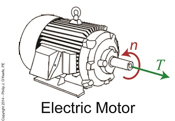
Last time we learned that we can get more torque out of a motor by using one of two methods. In the first method we attach a gear train to the motor, then try different gear sizes until we arrive at the desired torque for the application. In the second method we eliminate the gear train altogether and simply use a higher horsepower motor to give us the torque we need. Today we’ll explore the second method. We’ll use the equation presented in our last blog to determine torque, T, relative to a motor’s horsepower, HP, when the motor operates at a speed, n: T = [HP ÷ n] × 63,025 In earlier blogs in this series we employed a gear train attached to an electric motor to power a lathe. It provided an insufficient 200 inch pounds of torque when 275 is required. Let’s use the equation and a little algebra to see how much horsepower this motor develops if it turns at a speed of 1750 RPM, a common speed for alternating current (AC) motors: 200 inch pounds = [HP ÷ 1750 RPM] × 63,025 200 = HP × 36.01 HP = 200 ÷ 36.01 = 5.55 horsepower For the purpose of our example today, let’s say we’ve nonsensically decided not to use a gear train, leaving us with no choice but to replace the underpowered motor with a more powerful one. So let’s see what size motor we’ll need to provide us with the required horsepower of 275 inch pounds. Using the torque equation and plugging in numbers already provided our equation becomes: 275 inch pounds = [HP ÷1750 RPM] × 63,025 275 = HP × 36.01 HP = 275 ÷ 36.01 = 7.64 horsepower This tells us that we need to replace the 5.55 horsepower motor with a 7.65 horsepower motor. As you might have guessed, the higher the motor’s horsepower, the larger that motor’s size and weight — if you’re not using a gear train, that is. Bigger, bulkier motors cost more to purchase and operate and also take up more space, which often makes them impractical to use. All this translates to the reality that sometimes it just makes more sense to use a gear train to provide more torque. It’s a lot easier and cheaper to attach a gear train to a motor and manipulate its gear sizes to arrive at desired torque than it is to buy a bigger motor. You may have deduced by now that it’s relatively easy to get more torque. Almost too easy. Next time we’ll see how increased torque comes at another type of cost, the cost of speed. _______________________________________
|

The Mathematical Link Between Gears in a Gear Train
Wednesday, May 14th, 2014|
Last time we analyzed the angular relationship between the Force and Distance vectors in this simple gear train. Today we’ll discover a commonality between the two gears in this train which will later enable us to develop individual torque calculations for them.
From the illustration it’s clear that the driving gear is mechanically linked to the driven gear by their teeth. Because they’re linked, force, and hence torque, is transmitted by way of the driving gear to the driven gear. Knowing this we can develop a mathematical equation to link the driving gear Force vector F1 to the driven gear Force vector F2, then use that linking equation to develop a separate torque formula for each of the gears in the train. We learned in the previous blog in this series that F1 and F2 travel in opposite directions to each other along the same line of action. As such, both of these Force vectors are situated in the same way so that they are each at an angle value ϴ with respect to their Distance vectors D1 and D2. This fact allows us to build an equation with like terms, and that in turn allows us to use trigonometry to link the two force vectors into a single equation: F = [F1 × sin(ϴ)] – [F2 × sin(ϴ)] where F is called a resultant Force vector, so named because it represents the force that results when the dead, or inert, weight that’s present in the resisting force F2 cancels out some of the positive force of F1. Next week we’ll simplify our gear train illustration and delve into more math in order to develop separate torque computations for each gear in the train. _______________________________________ |


