Archive for the ‘Product Liability’ Category
Monday, August 21st, 2017
|
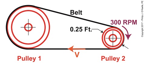
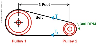
Last time we developed an equation to compute tangential velocity, V, of the belt in our example pulley and belt system. Today we’ll plug numbers into this equation and arrive at a numerical value for this belt velocity.
Belt Velocity
The equation we’ll be working with is,
V = π × D2 ÷ t2 (1)
where, D2 is the diameter of Pulley 2 and π represents the constant 3.1416. We learned that Pulley 2’s period of revolution, t2, is related to its rotational speed, N2, which represents the time it takes for it to make one revolution and is represented by this equation,
N2 = 1 ÷ t2 (2)
We’ll now solve for the belt’s velocity, V, using known values, starting off with rearranging terms so we can solve for t2,
t2 = 1 ÷ N2 (3)
We were previously given that N2 is 300 RPM, or revolutions per minute, so equation (3) becomes,
t2 = 1 ÷ 300 RPM = 0.0033 minutes (4)
This tells us that Pulley 2 takes 0.0033 minutes to make one revolution in our pulley-belt assembly.
Pulley 2’s diameter, D2, was previously determined to be 0.25 feet. Inserting this value equation (1) becomes,
V = π × (0.25 feet) ÷ (0.0033 minutes) (5)
V = 237.99 feet/minute (6)
We’ve now determined that the belt in our pulley-belt assembly zips around at a velocity of 237.99 feet per minute.
Next time we’ll apply this value to equation (6) and determine the belt’s tight side tension, T1.
Copyright 2017 – Philip J. O’Keefe, PE
Engineering Expert Witness Blog
____________________________________ |
Tags: belt, belt velocity, loose side tension, minimum belt width, period of revolution, pulley, pulley and belt system, pulley diameter, pulley rotational speed, tangential velocity
Posted in Engineering and Science, Expert Witness, Forensic Engineering, Innovation and Intellectual Property, Personal Injury, Product Liability | Comments Off on Belt Velocity
Monday, August 14th, 2017
|
Last time we introduced the Mechanical Power Formula, which is used to compute power in pulley-belt assemblies, and we got as far as introducing the term tangential velocity, V, a key variable within the Formula. Today we’ll devise a new formula to compute this tangential velocity.
Our starting point is the formula introduced last week to compute the amount of power, P, in our pulley-belt example is, again,
P = (T1 – T2) × V (1)
We already know that P is equal to 4 horsepower, we have yet to determine the belt’s tight side tension, T1, and loose side tension, T2, and of course V, the formula for which we’ll develop today.
Tangential Velocity
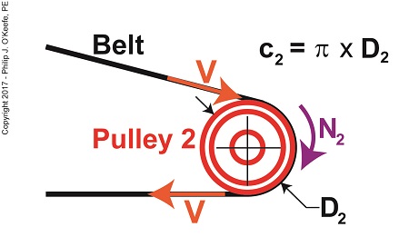
Tangential velocity is dependent on both the circumference, c2, and rotational speed, N2, of Pulley 2. The circumference represents the length of Pulley 2’s curved surface. The belt travels part of this distance as it makes its way from Pulley 2 back to Pulley 1. The rotational speed, N2, represents the rate that it takes for Pulley 2’s curved surface to make one revolution while propelling the belt. This time period is known as the period of revolution, t2, and is related to N2 by this equation,
N2 = 1 ÷ t2 (2)
The rotational speed of Pulley 2 is specified in our example as 300 RPMs, or revolutions per minute, and we’ll denote that speed as N2 in light of the fact it’s referring to speed present at the location of Pulley 2. As we build the formula, we’ll be converting N2 into velocity, specifically tangential velocity, V, which is the velocity at which the belt operates, this in turn will enable us to solve equation (1).
Why speak in terms of tangential velocity rather than plain old ordinary velocity? Because the moving belt’s orientation to the surface of the pulley lies at a tangent in relation to the pulley’s circumference, c2, as shown in the above illustration. Put another way, the belt enters and leaves the curved surface of the pulley in a straight line.
Generally speaking, velocity is distance traveled over a period of time, and tangential velocity is no different. So taking time into account we arrive at this formula,
V = c2 ÷ t2 (3)
Since the surface of Pulley 2 is a circle, its circumference can be computed using a formula developed thousands of years ago by the Greek engineer and mathematician Archimedes. It is,
c2 = π × D2 (4)
where D2 is the diameter of the pulley and π represents the constant 3.1416.
We now arrive at the formula for tangential velocity by combining equations (3) and (4),
V = π × D2 ÷ t2 (5)
Next time we’ll plug numbers into equation (5) and solve for V.
Copyright 2017 – Philip J. O’Keefe, PE
Engineering Expert Witness Blog
____________________________________ |
Tags: belt, belt velocity, circumference, engineer, loose side tension, mechanical power formula, period of revolution, pulley, pulleys, speed, tangential velocity, tight side tension, velocity
Posted in Engineering and Science, Expert Witness, Forensic Engineering, Innovation and Intellectual Property, Personal Injury, Product Liability | Comments Off on Tangential Velocity
Saturday, July 29th, 2017
|
Last time we determined the value for one of the key variables in the Euler-Eytelwein Formula known as the angle of wrap. To do so we worked with the relationship between the two tensions present in our example pulley-belt assembly, T1 and T2. Today we’ll use physics to solve for T2 and arrive at the Mechanical Power Formula, which enables us to compute the amount of power present in our pulley and belt assembly, a common engineering task.
To start things off let’s reintroduce the equation which defines the relationship between our two tensions, the Euler-Eytelwein Formula, with the value for e, Euler’s Number, and its accompanying coefficients, as determined from our last blog,
T1 = 2.38T2 (1)
Before we can calculate T1 we must calculate T2. But before we can do that we need to discuss the concept of power.
The Mechanical Power Formula in Pulley and Belt Assemblies
Generally speaking, power, P, is equal to work, W, performed per unit of time, t, and can be defined mathematically as,
P = W ÷ t (2)
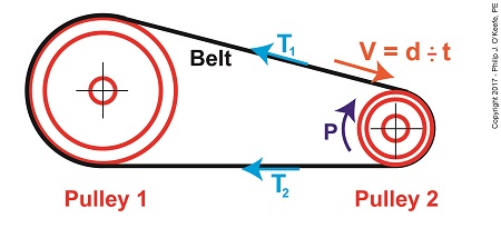
Now let’s make equation (2) specific to our situation by converting terms into those which apply to a pulley and belt assembly. As we discussed in a past blog, work is equal to force, F, applied over a distance, d. Looking at things that way equation (2) becomes,
P = F × d ÷ t (3)
In equation (3) distance divided by time, or “d ÷ t,” equals velocity, V. Velocity is the distance traveled in a given time period, and this fact is directly applicable to our example, which happens to be measured in units of feet per second. Using these facts equation (3) becomes,
P = F × V (4)
Equation (4) contains variables that will enable us to determine the amount of mechanical power, P, being transmitted in our pulley and belt assembly.
The force, F, is what does the work of transmitting mechanical power from the driving pulley, pulley 2, to the passive driven pulley, pulley1. The belt portion passing through pulley 1 is loose but then tightens as it moves through pulley 2. The force, F, is the difference between the belt’s tight side tension, T1, and loose side tension, T2. Which brings us to our next equation, put in terms of these two tensions,
P = (T1 – T2) × V (5)
Equation (5) is known as the Mechanical Power Formula in pulley and belt assemblies.
The variable V, is the velocity of the belt as it moves across the face of pulley 2, and it’s computed by yet another formula. We’ll pick up with that issue next time.
Copyright 2017 – Philip J. O’Keefe, PE
Engineering Expert Witness Blog
____________________________________ |
Tags: belt, distance divided by time, engineering, Euler-Eytelwein Formula, Euler's Number, force, loose side tension, mechanical power, mechanical power formula, power, power transmitted, pulley, tight side tension, velocity, work
Posted in Engineering and Science, Expert Witness, Forensic Engineering, Innovation and Intellectual Property, Personal Injury, Product Liability | Comments Off on The Mechanical Power Formula in Pulley and Belt Assemblies
Monday, July 17th, 2017
|
Sometimes things which appear simple turn out to be rather complex. Such is the case with the Euler-Eytelwein Formula, a small formula with a big job. It computes how friction, an omnipresent phenomenon in mechanical assemblies, contributes to the transmission of mechanical power. Today we’ll determine the value of one of the Euler-Eytelwein Formula’s variables, the angle of wrap.
Determining Angle of Wrap
Here again is the basis for our calculations, the Euler-Eytelwein Formula.
T1 = T2 × e(μθ) (1)
To recap what we’ve discussed thus far, T1 is the tight side tension, the maximum the belt can endure before breaking. T2 is the loose side tension. It’s just going along for the ride. The term e is Euler’s Number, a constant equal to 2.718, and the coefficient of friction, μ, for contact points between the belt and pulleys is 0.3 based on their materials.
The formula introduced last time to calculate the angle of wrap, θ, is,
θ = (180 – 2α) × (π ÷ 180) (2)
where,
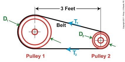
α = sin-1((D1 – D2) ÷ 2x) (3)
By direct measurement we’ve determined the pulleys’ diameters, D1 and D2, are equal to 1 foot and 0.25 feet respectively. The term x is the distance between the two pulley shafts, 3 feet. The term sin-1 is a trigonometric function known as inverse sine, a button commonly found on scientific calculators.
Inserting our known values into equation (3) we arrive at,
α = sin-1((1.0 foot – 0.25 feet) ÷ 2 × (3 feet)) (4)
α = 7.18 (5)
We can now incorporate equation (5) into equation (2) to solve for θ,
θ = (180 – (2 × 7.18)) × (π ÷ 180) (6)
θ = 2.89 (7)
Inserting the values for m and θ into equation (1) we arrive at,
T1 = T2 × 2.718(0.3 × 2.89) (8)
T1 = 2.38T2 (9)
We have at this point solved for over half of the unknown variables in the Euler-Eytelwein Formula. We still can’t solve for T1, because we don’t know the value of T2. But that will change next time when we introduce yet another formula, this one to determine the amount of mechanical power present in our pulley-belt system.
Copyright 2017 – Philip J. O’Keefe, PE
Engineering Expert Witness Blog
____________________________________ |
Tags: angle of wrap, belt, coefficient of friction, Euler-Eytelwein Formula, Euler's Number, friction, loose side tension, mechanical assemblies, mechanical power, pulley, pullies, tight side tension
Posted in Engineering and Science, Expert Witness, Forensic Engineering, Innovation and Intellectual Property, Personal Injury, Product Liability | Comments Off on Determining Angle of Wrap
Wednesday, July 5th, 2017
|
Last time we introduced a scenario involving a hydroponics plant powered by a gas engine and multiple pulleys. Connecting the pulleys is a flat leather belt. Today we’ll take a step further towards determining what width that belt needs to be to maximize power transmission efficiency. We’ll begin by revisiting the two T’s of the Euler-Eytelwein Formula and introducing a formula to determine a key variable, angle of wrap.
The Angle of Wrap Formula
We must start by calculating T1, the tight side tension of the belt, which is the maximum tension the belt is subjected to. We can then calculate the width of the belt using the manufacturer’s specified safe working tension of 300 pounds per inch as a guide. But first we’ll need to calculate some key variables in the Euler-Eytelwein Formula, which is presented here again,
T1 = T2× e(μθ) (1)
We determined last time that the coefficient of friction, μ, between the two interfacing materials of the belt and pulley are, respectively, leather and cast iron, which results in a factor of 0.3.
The other factor shown as a exponent of e is the angle of wrap, θ, and is calculated by the formula,
θ = (180 – 2α) × (π ÷ 180) (2)
You’ll note that this formula contains some unique terms of its own, one of which is familiar, namely π, the other, α, which is less familiar. The unnamed variable α is used as shorthand notation in equation (2), to make it shorter and more manageable. It has no particular significance other than the fact that it is equal to,
α = sin-1((D1 – D2) ÷ 2x) (3)
If we didn’t use this shorthand notation for α, equation (2) would be written as,
θ = (180 – 2(sin-1((D1 – D2) ÷ 2x))) × (π ÷ 180) (3a)
That’s a lot of parentheses!
Next week we’ll get into some trigonometry when we discuss the diameters of the pulleys, which will allow us to solve for the angle of wrap.
Copyright 2017 – Philip J. O’Keefe, PE
Engineering Expert Witness Blog
____________________________________ |
Tags: angle of wrap, belt, belt tension, coefficient of friction, Euler-Eytelwein Formula, mechanical power transmission, pulley, pulleys
Posted in Engineering and Science, Expert Witness, Forensic Engineering, Innovation and Intellectual Property, Personal Injury, Product Liability | Comments Off on The Angle of Wrap Formula
Friday, June 23rd, 2017
|
Belts are important. They make fashion statements, hold things up, keep things together. Today we’re introducing a scenario in which the Euler-Eytelwein Formula will be used to, among other things, determine the ideal width of a belt to be used in a mechanical power transmission system consisting of two pulleys inside a hydroponics plant. The ideal width belt would serve to maximize friction between the belt and pulleys, thus controlling slippage and maximizing belt strength to prevent belt breakage.
An engineer is tasked with designing an irrigation system for a hydroponics plant. Pulley 1 is connected to the shaft of a water pump, while Pulley 2 is connected to the shaft of a small gasoline engine.
What Belt Width does a Hydroponics Plant Need?
Mechanical power is transmitted by the belt from the engine to the pump at a constant rate of 4 horsepower. The belt material is leather, and the two pulleys are made of cast iron. The coefficient of friction, μ, between these two materials is 0.3, according to Marks Standard Handbook for Mechanical Engineers. The belt manufacturer specifies a safe working tension of 300 pounds force per inch width of the belt. This is the maximum tension the belt can safely withstand before breaking.
We’ll use this information to solve for the ideal belt width to be used in our hydroponics application. But first we’re going to have to re-visit the two T’s of the Euler-Eytelwein Formula. We’ll do that next time.
Copyright 2017 – Philip J. O’Keefe, PE
Engineering Expert Witness Blog
____________________________________ |
Tags: belt, belt breakage, coefficient of friction, engine, engineer, horsepower, leather belt, mechanical power transmission, pulley, pump
Posted in Engineering and Science, Expert Witness, Forensic Engineering, Innovation and Intellectual Property, Personal Injury, Product Liability | Comments Off on What Belt Width does a Hydroponics Plant Need?
Tuesday, June 13th, 2017
|
Last week we saw how friction coefficients as used in the Euler-Eyelewein Formula, can be highly specific to a specialized application, U.S. Navy ship capstans. In fact, many diverse industries benefit from aspects of the Euler-Eytelwein Formula. Today we’ll introduce another engineering application of the Formula, exploring its use within the irrigation system of a hydroponics plant.
Another Specialized Application of the Euler-Eyelewein Formula
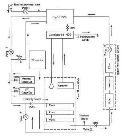
Pumps conveying water are an indispensable part of a hydroponics plant. In the schematic shown here they are portrayed by the symbol ⊗.
In our simplified scenario to be presented next week, these pumps are powered by a mechanical power transmission system, each consisting of two pulleys and a belt. One pulley is connected to a water pump, the other pulley to a gasoline engine. A belts runs between the pulleys to deliver mechanical power from the engine to the pump.
The width of the belts is a key component in an efficiently running hydroponics plant. We’ll see how and why that’s so next time.
Copyright 2017 – Philip J. O’Keefe, PE
Engineering Expert Witness Blog
____________________________________ |
Tags: belt, belt width, coefficient of friction, engineering, Euler-Etytelwein Formula, gasoline engine, hydroponics, mechanical power transmission, power, pulley, pump
Posted in Engineering and Science, Expert Witness, Forensic Engineering, Innovation and Intellectual Property, Personal Injury, Product Liability, Professional Malpractice | Comments Off on Another Specialized Application of the Euler-Eyelewein Formula
Sunday, June 4th, 2017
|
We’ve been talking about pulleys for awhile now, and last week we introduced the term friction coefficient, numerical values derived during testing which quantify the amount of friction present when different materials interact. Friction coefficients for common materials are routinely presented in engineering texts like Marks’ Standard Handbook for Mechanical Engineers. But there are circumstances when more specificity is required, such as when the U.S. Navy, more specifically the Navy Material Command, tested the interaction between various synthetic ropes and ship capstans and developed their own specialized friction coefficients in the process.
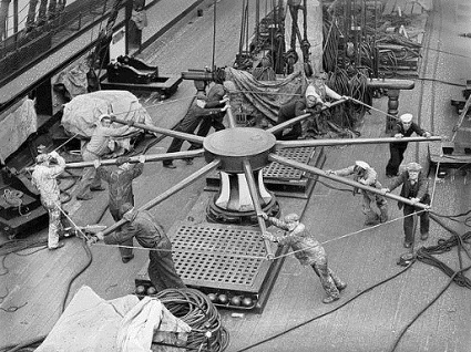
Navy Capstans and the Development of Specialized Friction Coefficients
Capstans are similar to pulleys but have one key difference, they’re made so rope can be wound around them multiple times. When the Navy set out to determine which synthetic rope worked best with their capstans, they did testing and developed highly specialized friction coefficients in the process. This research was at one time Top Secret but has now been declassified. To read more about it, follow this link to the actual handbook:
https://archive.org/stream/DTIC_ADA036718#page/n0/mode/2up
Copyright 2017 – Philip J. O’Keefe, PE
Engineering Expert Witness Blog
____________________________________ |
Tags: capstan, engineering, friction, friction coefficient, pulley, rope
Posted in Engineering and Science, Expert Witness, Forensic Engineering, Innovation and Intellectual Property, Personal Injury, Product Liability | Comments Off on Navy Capstans and the Development of Specialized Friction Coefficients
Sunday, May 14th, 2017
|
Last time we introduced some of the variables in the Euler-Eytelwein Formula, an equation used to examine the amount of friction present in pulley-belt assemblies. Today we’ll explore its two tension-denoting variables, T1 and T2.
Here again is the Euler-Eytelwin Formula,where, T1 and T2 are belt tensions on either side of a pulley,
T1 = T2 × e(μθ)
T1 is known as the tight side tension of the assembly because, as its name implies, the side of the belt containing this tension is tight, and that is so due to its role in transmitting mechanical power between the driving and driven pulleys. T2 is the loose side tension because on its side of the pulley no mechanical power is transmitted, therefore it’s slack–it’s just going along for the ride between the driving and driven pulleys.
Due to these different roles, the tension in T1 is greater than it is in T2.
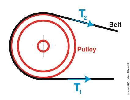
The Two T’s of the Euler-Eytelwein Formula
In the illustration above, tension forces T1 and T2 are shown moving in the same direction, because the force that keeps the belt taught around the pulley moves outward and away from the center of the pulley.
According to the Euler-Eytelwein Formula, T1 is equal to a combination of factors: tension T2 ; the friction that exists between the belt and pulley, denoted as μ; and how much of the belt is in contact with the pulley, namely θ.
We’ll get into those remaining variables next time.
Copyright 2017 – Philip J. O’Keefe, PE
Engineering Expert Witness Blog
____________________________________ |
Tags: belt, belt tension, driven pulley, driving pulley, engineering, Euler-Eytelwein Formula, mechanical power transmission, pulley
Posted in Engineering and Science, Expert Witness, Forensic Engineering, Innovation and Intellectual Property, Personal Injury, Product Liability | Comments Off on The Two T’s of the Euler-Eytelwein Formula
Friday, May 5th, 2017
|
Last time we introduced the Pulley Speed Ratio Formula, a Formula which assumes a certain amount of friction in a pulley-belt assembly in order to work. Today we’ll introduce another Formula, one which oversees how friction comes into play between belts and pulleys, the Euler-Eytelwein Formula. It’s a Formula developed by two pioneers of engineering introduced in an earlier blog, Leonhard Euler and Johann Albert Eytelwein.
Here again is the Pulley Speed Ratio Formula,
D1 × N1 = D2 × N2
where, D1 is the diameter of the driving pulley and D2 the diameter of the driven pulley. The pulleys’ rotational speeds are represented by N1 and N2.
This equation works when it operates under the assumption that friction between the belt and pulleys is, like Goldilock’s preferred bed, “just so.” Meaning, friction present is high enough so the belt doesn’t slip, yet loose enough so as not to bring the performance of a rotating piece of machinery to a grinding halt.
Ideally, you want no slippage between belt and pulleys, but the only way for that to happen is if you have perfect friction between their surfaces—something that will never happen because there’s always some degree of slippage. So how do we design a pulley-belt system to maximize friction and minimize slip?
Before we get into that, we must first gain an understanding of how friction comes into play between belts and pulleys. To do so we’ll use the famous Euler-Eytelwein Formula, shown here,
A First Look at the Euler-Eytelwein Formula
where, T1 and T2 are belt tensions on either side of a pulley.
We’ll continue our exploration of the Euler-Eytelwein Formula next time when we discuss the significance of its two sources of tension.
Copyright 2017 – Philip J. O’Keefe, PE
Engineering Expert Witness Blog
____________________________________ |
Tags: belt, belt slippage, belt tension, drive belt, engineering, Euler-Eytelwein Formula, friction, mechanical power transmission, pulley, pulley belt system
Posted in Engineering and Science, Expert Witness, Forensic Engineering, Innovation and Intellectual Property, Personal Injury, Product Liability | Comments Off on A First Look at the Euler-Eytelwein Formula