May 25th, 2017
|
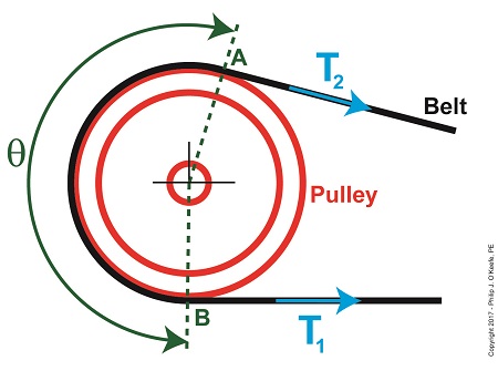
Last time we learned that the two T’s in the Euler-Eytelwein Formula correspond to different belt tensions on either side of a pulley wheel in a pulley-belt assembly. Today we’ll see what the remaining variables in this famous Formula are all about, paying special attention to the angle of wrap that’s formed by the belt wrapping around the pulley wheel.
Angle of Wrap in the Euler-Eytelwein Formula
Here again is the Euler-Eytelwein Formula,
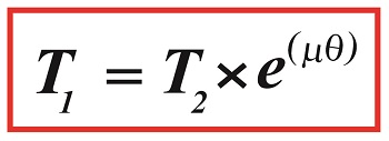
T1 = T2 × e(μθ)
The tight side tension, T1, is equal to a combination of factors, namely: loose side tension T2 ; the friction that exists between the belt and pulley, denoted as μ ; and the length of belt coming in direct contact with the pulley, namely, θ. These last two terms are exponents of the term, e, known as Euler’s Number, a mathematical constant used in many circles, including science, engineering, and economics, to calculate a wide variety of things, from bell curves to compound interest rates. It’s a rather esoteric term, much like the term π that’s used to calculate values associated with circles.
Euler’s Number was discovered in 1683 by Swiss mathematician Jacob Bernoulli, but oddly enough was named after Leonhard Euler. Its value, 2.718, was determined while Bernoulli manipulated high level mathematics to calculate compound interest rates. If you’d like to learn more about that, follow this link.
The term μ is known as the friction coefficient. It quantifies the degree of friction, or roughness, present between the belt and pulley where they make contact. It’s a specific number that remains constant for a given combination of materials. For example, according to Marks’ Standard Handbook for Mechanical Engineers, the value of μ for a leather belt operating on an iron pulley is 0.38. The numerical values for these coefficients were determined over the last few centuries by engineers conducting laboratory testing on various belt and pulley materials. They’re now routinely found in a variety of engineering texts and handbooks.
Finally, the term θ denotes the angle of wrap that the belt makes while in contact with the face of the pulley. In our example illustration above, θ measures the arc that’s formed by the belt riding along the surface of the pulley between points A and B, as shown by dotted lines. The angle of wrap is important to overall functionality of the assembly, because the proper amount of friction will allow the pulley-belt assembly to operate efficiently and without slippage.
Next time we’ll present an example and use the Euler-Eytelwein Formula to calculate optimal belt friction within a pulley-belt assembly.
Copyright 2017 – Philip J. O’Keefe, PE
Engineering Expert Witness Blog
____________________________________ |
Posted in Engineering and Science | Comments Off on Angle of Wrap in the Euler-Eytelwein Formula
May 14th, 2017
|
Last time we introduced some of the variables in the Euler-Eytelwein Formula, an equation used to examine the amount of friction present in pulley-belt assemblies. Today we’ll explore its two tension-denoting variables, T1 and T2.
Here again is the Euler-Eytelwin Formula,where, T1 and T2 are belt tensions on either side of a pulley,
T1 = T2 × e(μθ)
T1 is known as the tight side tension of the assembly because, as its name implies, the side of the belt containing this tension is tight, and that is so due to its role in transmitting mechanical power between the driving and driven pulleys. T2 is the loose side tension because on its side of the pulley no mechanical power is transmitted, therefore it’s slack–it’s just going along for the ride between the driving and driven pulleys.
Due to these different roles, the tension in T1 is greater than it is in T2.
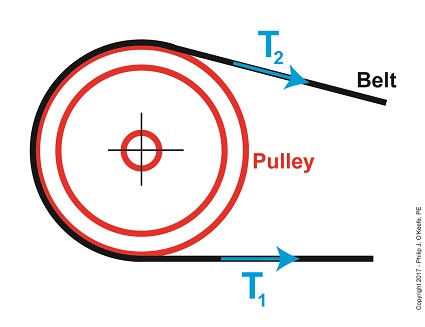
The Two T’s of the Euler-Eytelwein Formula
In the illustration above, tension forces T1 and T2 are shown moving in the same direction, because the force that keeps the belt taught around the pulley moves outward and away from the center of the pulley.
According to the Euler-Eytelwein Formula, T1 is equal to a combination of factors: tension T2 ; the friction that exists between the belt and pulley, denoted as μ; and how much of the belt is in contact with the pulley, namely θ.
We’ll get into those remaining variables next time.
Copyright 2017 – Philip J. O’Keefe, PE
Engineering Expert Witness Blog
____________________________________ |
Tags: belt, belt tension, driven pulley, driving pulley, engineering, Euler-Eytelwein Formula, mechanical power transmission, pulley
Posted in Engineering and Science, Expert Witness, Forensic Engineering, Innovation and Intellectual Property, Personal Injury, Product Liability | Comments Off on The Two T’s of the Euler-Eytelwein Formula
May 5th, 2017
|
Last time we introduced the Pulley Speed Ratio Formula, a Formula which assumes a certain amount of friction in a pulley-belt assembly in order to work. Today we’ll introduce another Formula, one which oversees how friction comes into play between belts and pulleys, the Euler-Eytelwein Formula. It’s a Formula developed by two pioneers of engineering introduced in an earlier blog, Leonhard Euler and Johann Albert Eytelwein.
Here again is the Pulley Speed Ratio Formula,
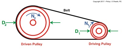
D1 × N1 = D2 × N2
where, D1 is the diameter of the driving pulley and D2 the diameter of the driven pulley. The pulleys’ rotational speeds are represented by N1 and N2.
This equation works when it operates under the assumption that friction between the belt and pulleys is, like Goldilock’s preferred bed, “just so.” Meaning, friction present is high enough so the belt doesn’t slip, yet loose enough so as not to bring the performance of a rotating piece of machinery to a grinding halt.
Ideally, you want no slippage between belt and pulleys, but the only way for that to happen is if you have perfect friction between their surfaces—something that will never happen because there’s always some degree of slippage. So how do we design a pulley-belt system to maximize friction and minimize slip?
Before we get into that, we must first gain an understanding of how friction comes into play between belts and pulleys. To do so we’ll use the famous Euler-Eytelwein Formula, shown here,
A First Look at the Euler-Eytelwein Formula
where, T1 and T2 are belt tensions on either side of a pulley.
We’ll continue our exploration of the Euler-Eytelwein Formula next time when we discuss the significance of its two sources of tension.
Copyright 2017 – Philip J. O’Keefe, PE
Engineering Expert Witness Blog
____________________________________ |
Tags: belt, belt slippage, belt tension, drive belt, engineering, Euler-Eytelwein Formula, friction, mechanical power transmission, pulley, pulley belt system
Posted in Engineering and Science, Expert Witness, Forensic Engineering, Innovation and Intellectual Property, Personal Injury, Product Liability | Comments Off on A First Look at the Euler-Eytelwein Formula
April 21st, 2017
|
Last time we saw how pulley diameter governs speed in engineering scenarios which make use of a belt and pulley system. Today we’ll see how this phenomenon is defined mathematically through application of the Pulley Speed Ratio Formula, which enables precise pulley diameters to be calculated to achieve specific rotational speeds. Today we’ll apply this Formula to a scenario involving a building’s ventilating system.
The Pulley Speed Ratio Formula is,
D1 × N1 = D2 × N2 (1)
where, D1 is the diameter of the driving pulley and D2 the diameter of the driven pulley.
A Pulley Speed Ratio Formula Application
The pulleys’ rotational speeds are represented by N1 and N2, and are measured in revolutions per minute (RPM).
Now, let’s apply Equation (1) to an example in which a blower must deliver a specific air flow to a building’s ventilating system. This is accomplished by manipulating the ratios between the driven pulley’s diameter, D2, with respect to the driving pulley’s diameter, D1. If you’ll recall from our discussion last time, when both the driving and driven pulleys have the same diameter, the entire assembly moves at the same speed, and this would be bad for our scenario.
An electric motor and blower impeller moving at the same speed is problematic because electric motors are designed to spin at much faster speeds than typical blower impellers in order to produce desired air flow. If their pulleys’ diameters were the same size, it would result in an improperly working ventilating system in which air passes through the furnace heat exchanger and air conditioner cooling coils far too quickly to do an efficient job of heating or cooling.
To bear this out, let’s suppose we have an electric motor turning at a fixed speed of 3600 RPM and a belt-driven blower with an impeller that must turn at 1500 RPM to deliver the required air flow according to the blower manufacturer’s data sheet. The motor shaft is fitted with a pulley 3 inches in diameter. What pulley diameter do we need for the blower to turn at the manufacturer’s required 1500 RPM?
In this example known variables are D1 = 3 inches, N1 = 3600 RPM, and N2 = 1500 RPM. The diameter D2 is unknown. Inserting the known values into equation (1), we can solve for D2,
(3 inches) × (3600 RPM) = D2 × (1500 RPM) (2)
Simplified, this becomes,
D2 = 7.2 inches (3)
Next time we’ll see how friction affects our scenario.
Copyright 2017 – Philip J. O’Keefe, PE
Engineering Expert Witness Blog
____________________________________ |
Tags: belt, blower, blower impeller, cooling coils, drive belt, driven pulley, driving pulley, electric motor, engineering, heat exchanger, mechanical power transmission, pulley, pulley speed, Pulley Speed Ratio Formula, RPM, ventilating system
Posted in Engineering and Science, Expert Witness, Forensic Engineering, Innovation and Intellectual Property, Personal Injury, Product Liability | Comments Off on A Pulley Speed Ratio Formula Application
April 8th, 2017
|
Soon after the first pulleys were used with belts to transmit mechanical power, engineers such as Leonhard Euler and Johann Albert Eytelwein discovered that the diameter of the pulleys used determined the speed at which they rotated. This allowed for a greater diversity in mechanical applications. We’ll set up an examination of this phenomenon today.
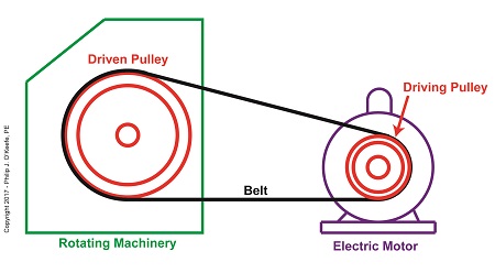
Last time we introduced this basic mechanical power transmission system consisting of a driving pulley, a driven pulley, and a belt, which we’ll call Situation A.
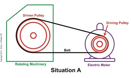
A Driven Pulley’s Larger Diameter Determines a Slower Speed
In this situation, the rotating machinery’s driven pulley diameter is larger than the electric motor’s driving pulley diameter. The result is the driven pulley turns at a slower speed than the driving pulley.
Now let’s say we need to speed the rotating machinery up so it produces more widgets per hour. In that case we’d make the driven pulley smaller, as shown in Situation B.
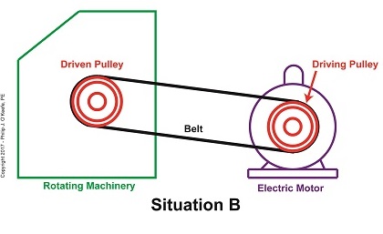
A Driven Pulley’s Smaller Diameter Determines a Faster Speed
With the smaller diameter driven pulley, the rotating machinery will operate faster than it did in Situation A.
Next week we’ll introduce the Pulley Speed Ratio Formula, which mathematically defines this phenomenon.
Copyright 2017 – Philip J. O’Keefe, PE
Engineering Expert Witness Blog
____________________________________ |
Tags: belt, driven pulley, driving pulley, electric motor, engineering, Johann Albert Eytelwein, Leonhard Euler, pulley diameter, Pulley Speed Ratio Formula, rotating machinery, rotational speed
Posted in Engineering and Science, Expert Witness, Forensic Engineering, Innovation and Intellectual Property, Personal Injury, Product Liability | Comments Off on Pulley Diameter Determines Speed
March 31st, 2017
|
Last time we introduced two historical legends in the field of engineering who pioneered the science of mechanical power transmission using belts and pulleys, Leonhard Euler and Johann Albert Eytelwein. Today we’ll build a foundation for understanding their famous Euler-Eytelwein Formula through our example of a simple mechanical power transmission system consisting of two pulleys and a belt, and in so doing demonstrate the difference between driven and driving pulleys.
Our example of a basic mechanical power transmission system consists of two pulleys connected by a drive belt. The driving pulley is attached to a source of mechanical power, for example, the shaft of an electric motor. The driven pulley, which is attached to the shaft of a piece of rotating machinery, receives the mechanical power from the electric motor so the machinery can perform its function.
The Difference Between Driven and Driving Pulleys
Next time we’ll see how driven pulleys can be made to spin at different speeds from the driving pulley, enabling different modes of operation in mechanical devices.
Copyright 2017 – Philip J. O’Keefe, PE
Engineering Expert Witness Blog
____________________________________ |
Tags: belt, driven pulley, driving pulley, electric motor, engineering, Euler, Euler-Eytelwein Formula, Eytelwein, mechanical power, mechanical power transmission, pulley, pulley speed, rotating machinery
Posted in Engineering and Science, Expert Witness, Forensic Engineering, Innovation and Intellectual Property, Personal Injury, Product Liability | Comments Off on The Difference Between Driven and Driving Pulleys
March 20th, 2017
|
They say necessity is the mother of invention, and today’s look at an influential historical figure in engineering bears that out. Last week we introduced Leonhard Euler and touched on his influence to the science of pulleys. Today we’ll introduce his contemporary and partner in science, Johann Albert Eytelwein, a German mathematician and visionary, a true engineering trailblazer whose contributions to the blossoming discipline of engineering led to later studies with pulleys.
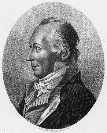
Johann Albert Eytelwein, Engineering Trailblazer
Johann Albert Eytelwein’s experience as a civil engineer in charge of the dikes of former Prussia led him to develop a series of practical mathematical problems that would enable his subordinates to operate more effectively within their government positions. He was a trailblazer in the field of applied mechanics and their application to physical structures, such as the dikes he oversaw, and later to machinery. He was instrumental in the founding of Germany’s first university level engineering school in 1799, the Berlin Bauakademie, and served as director there while lecturing on many developing engineering disciplines of the time, including machine design and hydraulics. He went on to publish in 1801 one of the most influential engineering books of his time, entitled Handbuch der Mechanik (Handbook of the Mechanic), a seminal work which combined what had previously been mere engineering theory into a means of practical application.
Later, in 1808, Eytelwein expanded upon this work with his Handbuch der Statik fester Koerper (Handbook of Statics of Fixed Bodies), which expanded upon the work of Euler. In it he discusses friction and the use of pulleys in mechanical design. It’s within this book that the famous Euler-Eytelwein Formula first appears, a formula Eytelwein derived in conjunction with Euler. The formula delves into the usage of belts with pulleys and examines the tension interplay between them.
More on this fundamental foundation to the discipline of engineering next time, with a specific focus on pulleys.
Copyright 2017 – Philip J. O’Keefe, PE
Engineering Expert Witness Blog
____________________________________ |
Tags: bel, engineering, friction, Johann Albert Eytelwein, mechanical power transmission, pulley, pulleys
Posted in Engineering and Science, Expert Witness, Forensic Engineering, Personal Injury, Product Liability | Comments Off on Johann Albert Eytelwein, Engineering Trailblazer
March 9th, 2017
|
Last time we ended our blog series on pulleys and their application within engineering as aids to lifting. Today we’ll embark on a new focus series, pulleys used in mechanical devices. We begin with some history, a peek at Swiss scientist and mathematician Leonhard Euler, a historical figure credited to be perhaps the greatest mathematician of the 18th Century.

Leonhard Euler, a Historical Figure in Pulleys
Euler is so important to math, he actually has two numbers named after him. One is known simply as Euler’s Number, 2.7182, most often notated as e, the other Euler’s Constant, 0.57721, notated γ, which is a Greek symbol called gamma. In fact, he developed most math notations still in use today, including the infamous function notation, f(x), which no student of elementary algebra can escape becoming intimately familiar with.
Euler authored his first theoretical essays on the science and mathematics of pulleys after experimenting with combining them with belts in order to transmit mechanical power. His theoretical work became the foundation of the formal science of designing pulley and belt drive systems. And together with German engineer Johann Albert Eytelwein, Euler is credited with a key formula regarding pulley-belt drives, the Euler-Eytelwein Formula, still in use today, and which we’ll be talking about in depth later in this blog series.
We’ll talk more about Eytelwein, another important historical figure who worked with pulleys, next time.
Copyright 2017 – Philip J. O’Keefe, PE
Engineering Expert Witness Blog
____________________________________ |
Tags: belt and pulley drive systems, belts, engineering, Euler's Constant, Euler's Number, Johann Albert Eytelwein, Leonhard Euler, mechanical power transmission, pulleys
Posted in Engineering and Science, Expert Witness, Forensic Engineering, Innovation and Intellectual Property, Personal Injury, Product Liability | Comments Off on Leonhard Euler, a Historical Figure in Pulleys
February 28th, 2017
|
For some time now we’ve been analyzing the helpfulness of the engineering phenomena known as pulleys and we’ve learned that, yes, they can be very helpful, although they do have their limitations. One of those ever-present limitations is due to the inevitable presence of friction between moving parts. Like an unsummoned gremlin, friction will be standing by in any mechanical situation to put the wrench in the works. Today we’ll calculate just how much friction is present within the example compound pulley we’ve been working with.

So How Much Friction is Present in our Compound Pulley?
Last time we began our numerical demonstration of the inequality between a compound pulley’s work input, WI, and work output, WO, an inequality that’s due to friction in its wheels. We began things by examining a friction-free scenario and discovered that to lift an urn with a weight, W, of 40 pounds a distance, d1, of 2 feet above the ground, Mr. Toga exerts a personal effort/force, F, of 10 pounds to extract a length of rope, d2, of 8 feet.
In reality our compound pulley must contend with the effects of friction, so we know it will take more than 10 pounds of force to lift the urn, a resistance which we’ll notate FF. To determine this value we’ll attach a spring scale to Mr. Toga’s end of the rope and measure his actual lifting force, FActual, represented by the formula,
FActual = F + FF (1)
We find that FActual equals 12 pounds. Thus our equation becomes,
12 Lbs = 10 Lbs + FF (2)
which simplifies to,
2 Lbs = FF (3)
Now that we’ve determined values for all operating variables, we can solve for work input and then contrast our finding with work output,
WI = (F × d2) + (FF × d2) (4)
WI = (10 Lbs × 8 feet) + (2 Lbs × 8 feet) (5)
WI = 96 Ft-Lbs (6)
We previously calculated work output, WO to be 80 Ft-Lbs, so we’re now in a position to calculate the difference between work input and work output to be,
WI – WO = 16 Ft-Lbs (7)
It’s evident that the amount of work Mr. Toga puts into lifting his urn requires 16 more Foot-Pounds of work input effort than the amount of work output produced. This extra effort that’s required to overcome the pulley’s friction is the same as the work required to carry a weight of one pound a distance of 16 feet. We can thus conclude that work input does not equal work output in a compound pulley.
Next time we’ll take a look at a different use for pulleys beyond that of just lifting objects.
Copyright 2017 – Philip J. O’Keefe, PE
Engineering Expert Witness Blog
____________________________________ |
Tags: compound pulley, engineering, friction, pulley, work, work input, work output
Posted in Engineering and Science, Expert Witness, Forensic Engineering, Innovation and Intellectual Property, Personal Injury, Product Liability | Comments Off on So How Much Friction is Present in our Compound Pulley?
February 15th, 2017
|
Last time we began work on a numerical demonstration and engineering analysis of the inequality of work input and output as experienced by our example persona, an ancient Greek lifting an urn. Today we’ll get two steps closer to demonstrating this reality as we work a compound pulley’s numerical puzzle, shuffling equations like a Rubik’s Cube to arrive at values for two variables crucial to our analysis, d2, the length of rope he extracts from the pulley while lifting, and F, the force/effort required to lift the urn in an idealized situation where no friction exists.

A Compound Pulley’s Numerical Puzzle is Like a Rubik’s Cube
We’ll continue manipulating the work input equation, WI, as shown in Equation (1), along with derivative equations, breaking it down into parts, and handle the two terms within parentheses separately. Term one, (F × d2), corresponds to the force/effort/work required to lift the urn in an idealized no-friction world. It’ll be our focus today as it provides a springboard to solving for variables F and d2.
WI = (F × d2) + (FF × d2) (1)
Previously we learned that when friction is present, work output, WO, is equal to work input minus the work required to oppose friction while lifting. Mathematically that’s represented by,
WO = WI – (FF × d2) (2)
We also previously calculated WO to equal 80 Ft-Lbs. To get F and d2 into a relationship with terms we already know the value for, namely WO, we substitute Equation (1) into Equation (2) and arrive at,
80 Ft-Lbs = (F × d2) + (FF × d2) – (FF × d2) (3)
simplified this becomes,
80 Ft-Lbs = F × d2 (4)
To find the value of d2, we’ll return to a past equation concerning compound pulleys derived within the context of mechanical advantage, MA. That is,
d2 ÷ d1 = MA (5)
And because in our example four ropes are used to support the weight of the urn, we know that MA equals 4. We also know from last time that d1 equals 2 feet. Plugging these numbers into Equation (5) we arrive at a value for d2,
d2 ÷ 2 ft = 4 (6)
d2 = 4 × 2 ft (7)
d2 = 8 ft (8)
Substituting Equation (8) into Equation (4), we solve for F,
80 Ft-Lbs = F × 8 ft (9)
F = 10 Pounds (10)
Now that we know F and d2 we can solve for FF, the amount of extra effort required by man or machine to overcome friction in a compound pulley assembly. It’s the final piece in the numerical puzzle which will then allow us to compare work input to output.
Copyright 2017 – Philip J. O’Keefe, PE
Engineering Expert Witness Blog
____________________________________ |
Tags: compound pulley, engineering, friction, friction force, lifting force, work input, work output
Posted in Engineering and Science, Expert Witness, Forensic Engineering, Innovation and Intellectual Property, Personal Injury, Product Liability | Comments Off on A Compound Pulley’s Numerical Puzzle is Like a Rubik’s Cube