Posts Tagged ‘gravity’
Friday, October 14th, 2016
|
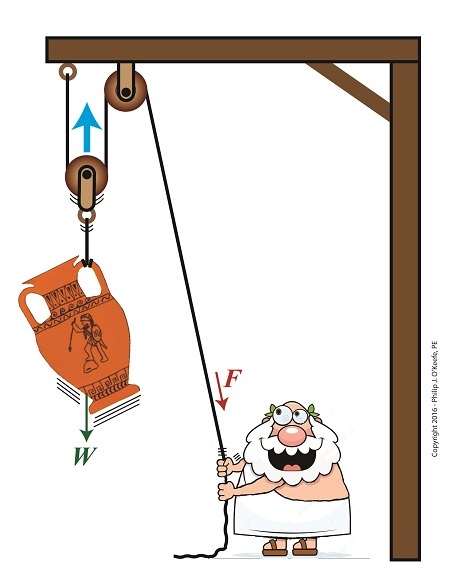
Last time we introduced the engineering concept of mechanical advantage, MA. Thanks to its presence in our compound pulley arrangement, it made a Grecian man’s job of holding an urn suspended in space twice as easy as compared to when he used a mere simple pulley. Today we’ll see what happens when our static scenario becomes active through dynamic lifting and how it affects his efforts.
Dynamic Lifting is Easier With a Compound Pulley
If you’ll recall from our last blog, Mr. Toga used a compound pulley to assist him in holding an urn stationary in space. To do so, he only needed to exert personal bicep force, F, equivalent to half the urn’s weight force, W, which meant he enjoyed a mechanical advantage of 2. Mathematically that is represented by,
F = W ÷ 2
If the urn weighs 40 pounds, then he only needs to exert 20 Lbs of personal effort to keep it suspended.
But when Mr. Toga uses more bicep power with that same compound pulley, he’s able to dynamically raise its position in space until it eventually meets with the beam that supports it. All the while he’ll be exerting a force greater than W ÷ 2. That relationship is represented by,
F > W ÷ 2
In the case of a 40 Lb urn, the lifting force Mr. Toga must exert to dynamically lift the urn is represented by,
F > 40 Lbs ÷ 2
F > 20 Lbs
where F represents a bicep force of at least 20 pounds. Fortunately for him, his efforts will never have to extend much beyond 20 Lbs of effort to lift the urn to the beam. That’s because gravity’s effect will remain nearly constant as the urn climbs, this being due to gravity’s influence upon objects decreasing by an insignificant amount over short distances above the Earth’s surface. As a matter of fact, at an altitude of 3,280 feet, gravity’s pull decreases by a mere 0.2 %.
The net result is that the compound pulley enables the same mechanical advantage whether a static or dynamic scenario exists, that is, regardless of whether Mr. Toga is simply holding the urn stationary in space or he’s actively tugging on his end of the rope to lift it higher.
Next time we’ll see how mechanical advantage increases when we add more fixed and moveable pulleys to our compound pulley arrangement.
Copyright 2016 – Philip J. O’Keefe, PE
Engineering Expert Witness Blog
____________________________________ |
Tags: compound pulley, dynamic lifting, engineering expert, force, gravity, gravity's pull, mechanical advantage, simple pulley, static, weight
Posted in Engineering and Science, Expert Witness, Forensic Engineering, Innovation and Intellectual Property, Personal Injury, Product Liability | Comments Off on Dynamic Lifting is Easier With a Compound Pulley
Friday, September 9th, 2016
|
Last time we introduced the compound pulley and saw how it improved upon a simple pulley, both of which I’ve engaged in my work as an engineering expert. Today we’ll examine the math behind the compound pulley. We’ll begin with a static representation and follow up with an active one in our next blog.
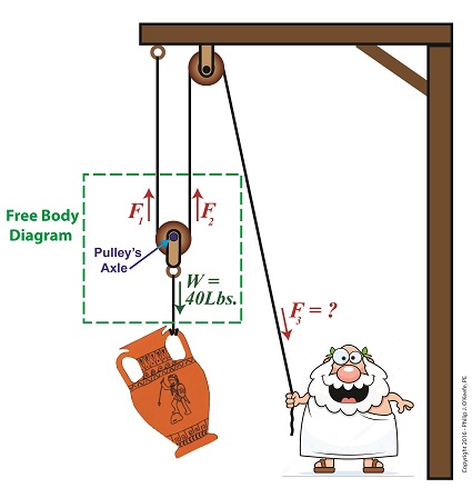
The compound pulley illustrated below contains three rope sections with three representative tension forces, F1, F2, and F3. Together, these three forces work to offset the weight, W, of a suspended urn weighing 40 lbs. Weight itself is a downward pulling force due to the effects of gravity.
To determine how our pulley scenario affects the man holding his section of rope and exerting force F3, we must first calculate the tension forces F1 and F2. To do so, we’ll use a free body diagram, shown in the green box, to display the forces’ relationship to one another.
The Math Behind a Static Compound Pulley
The free body diagram only takes into consideration the forces inside the green box, namely F1, F2, and W.
For the urn to remain suspended stationary in space, we know that F1 and F2 are each equal to one half the urn’s weight, because they’re spaced equidistant from the pulley’s axle, which directly supports the weight of the urn. Mathematically this looks like,
F1 = F2 = W ÷ 2
Because we know F1 and F2, we also know the value of F3, thanks to an engineering rule concerning pulleys. That is, when a single rope is used to support an object with pulleys, the tension force in each section of rope must be equal along the entire length of the rope, which means F1 = F2 = F3. This rule holds true whether the rope is threaded through one simple pulley or a complex array of fixed and moveable simple pulleys within a compound pulley. If it wasn’t true, then unequal tension along the rope sections would result in some sections being taut and others limp, which would result in a situation which would not make lifting the urn any easier and thereby defeat the purpose of using pulleys.
If the urn’s weight, W, is 40 pounds, then according to the aforementioned engineering rule,
F1 = F2 = F3= W ÷ 2
F1 = F2 = F3 = (40 pounds) ÷ 2 = 20 pounds
Mr. Toga needs to exert a mere 20 pounds of personal effort to keep the immobile urn suspended above the ground. It’s the same effort he exerted when using the improved simple pulley in a previous blog, but this time he can do it from the comfort and safety of standing on the ground.
Next time we’ll examine the math and mechanics behind an active compound pulley and see how movement affects F1 , F2 , and F3.
Copyright 2016 – Philip J. O’Keefe, PE
Engineering Expert Witness Blog
____________________________________ |
Tags: beam, compound pulley, engineering expert, fixed pulley, free body diagram, gravity, lifting, math, movable pulley, pulling, rope rule, simple pulley, tension force, weight force
Posted in Engineering and Science, Expert Witness, Forensic Engineering, Innovation and Intellectual Property, Personal Injury, Product Liability | Comments Off on The Math Behind a Static Compound Pulley
Tuesday, August 2nd, 2016
|
Last time we introduced the free body diagram, applied it to a simple pulley, and discovered that in so doing lifting objects required 50% less effort. As an engineering expert, I’ve sometimes put this improved version of a simple pulley to work for me in designs. We’ll do the math behind the improvement today.
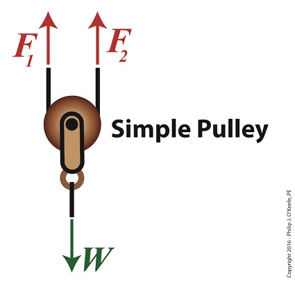
Here again is the free body diagram showing the improved simple pulley as introduced last week.
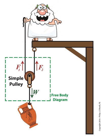
The Math Behind the Improved Simple Pulley
The illustration shows the three forces, F1, F2, and W, acting upon the simple pulley within the highlighted free body diagram. Forces F1 and F2 are exerted from above and act in opposition to the downward pull of gravity, represented by the weight of the urn, W. Forces F1 and F2 are produced by that which holds onto either end of the rope that’s threaded through the pulley. In our case those forces are supplied by a man in a toga and a beam. By engineering convention, these upward forces, F1 and F2, are considered positive, while the downward force, W, is negative.
In the arrangement shown in our illustration, the pulley’s rope ends equally support the urn’s weight, as demonstrated by the fact that the urn remains stationary in space, neither moving up nor down. In other words, forces F1 and F2 are equal.
Now, according to the basic rule of free body diagrams, the three forces F1, F2, and W must add up to zero in order for the pulley to remain stationary. Put another way, if the pulley isn’t moving up or down, the positive forces F1 and F2 are balancing the negative force presented by the urn’s weight, W. Mathematically this looks like,
F1 + F2 – W = 0
or, by rearranging terms,
F1 + F2 = W
We know that F1 equals F2, so we can substitute F1 for F2 in the preceding equation to arrive at,
F1 + F1 = W
or,
2 × F1 = W
Using algebra to divide both sides of the equation by 2, we get:
F1 = W ÷ 2
Therefore,
F1 = F2 = W ÷ 2
If the sum of the forces in a free body diagram do not equal zero, then the suspended object will move in space. In our situation the urn moves up if our toga-clad friend pulls on his end of the rope, and it moves down if Mr. Toga reduces his grip and allows the rope to slide through his hand under the influence of gravity.
The net real world benefit to our Grecian friend is that the urn’s 20-pound weight is divided equally between him and the beam. He need only apply a force of 10 pounds to keep the urn suspended.
Next time we’ll see how the improved simple pulley we’ve discussed today led to the development of the compound pulley, which enabled heavier objects to be lifted.
Copyright 2016 – Philip J. O’Keefe, PE
Engineering Expert Witness Blog
____________________________________ |
Tags: engineering expert, forces, free body diagram, gravity, pulley, simple pulley, weight
Posted in Engineering and Science, Expert Witness, Forensic Engineering, Innovation and Intellectual Property, Personal Injury, Product Liability | Comments Off on The Math Behind the Improved Simple Pulley
Thursday, July 21st, 2016
|
Sometimes the simplest alteration in design results in a huge improvement, a truth I’ve discovered more than a few times during my years as an engineering expert. Last time we introduced the simple pulley and revealed that its usefulness was limited to the strength of the pulling force behind it. Hundreds of years ago that force was most often supplied by a man and his biceps. But ancient Greeks found an ingenious and simple way around this limitation, which we’ll highlight today by way of a modern design engineer’s tool, the free body diagram.
Around 400 BC, the Greeks noticed that if they detached the simple pulley from the beam it was affixed to in our last blog and instead allowed it to be suspended in space with one of its rope ends fastened to a beam, the other rope end to a pulling force, something interesting happened.
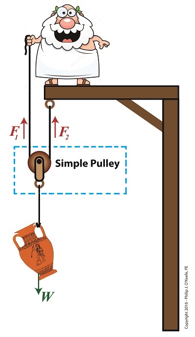
The Simple Pulley Improved
It was much easier to lift objects while suspended in air. As a matter of fact, it took 50% less effort. To understand why, let’s examine what engineers call a free body diagram of the pulley in our application, as shown in the blue inset box and in greater detail below.
Using a Free Body Diagram to Understand Simple Pulleys
The blue insert box in the first illustration highlights the subject at hand. A free body diagram helps engineers analyze forces acting upon a stationary object suspended in space. The forces acting upon the object, in our case a simple pulley, represent both positive and negative values. The free body diagram above indicates that forces pointing up are, by engineering convention, considered to be positive, while downward forces are negative. The basic rule of all free body diagrams is that in order for an object to remain suspended in a fixed position in space, the sum of all forces acting upon it must equal zero.
We’ll see how the free body diagram concept is instrumental in understanding the improvement upon the action of a simple pulley next time, when we attack the math behind it.
Copyright 2016 – Philip J. O’Keefe, PE
Engineering Expert Witness Blog
____________________________________ |
Tags: beam, engineering expert, engineers, force, free body diagram, gravity, pulley, pulling force, rope, simple pulley, weight force
Posted in Engineering and Science, Expert Witness, Forensic Engineering, Innovation and Intellectual Property, Personal Injury, Product Liability | Comments Off on Using a Free Body Diagram to Understand Simple Pulleys
Wednesday, September 2nd, 2015
|
Last time we calculated the potential energy hidden within a coffee mug resting on a shelf. The concept of a passive object possessing energy may not be something all readers can identify with, but the secret behind that mug’s latent energy lies within The Law of Conservation of Energy, the topic we’ll be discussing today.
Julius Robert von Mayer, a German physicist of the mid 19th Century, is the man behind the Law. He posited that energy cannot be created or destroyed, it can only be transferred from one object to another or converted from one form of energy to another. Forms of energy include potential, kinetic, heat, chemical, mechanical, and electrical, all of which have the ability to become another form of energy.
Let’s take our coffee mug for example. Where did its potential energy come from? Ultimately, from the radiant energy emitted by the sun. The sun’s radiant energy was absorbed by plants and then converted to chemical energy through the process of photosynthesis, enabling them to grow. When they were later eaten by humans and other animals, the plants’ chemical energy became incorporated into their bodies’ cells, including the arm muscles used to lift the mug to the shelf.
In the act of lifting the cup, the arm’s muscle cells converted their own chemical energy into mechanical energy. And because lifting a mug to a shelf is work, for some of us greater than others, some of the arm’s chemical energy became heat energy which was lost to the environment.
Because of the elevated perch provided to the mug by the arm, which was in direct defiance of Earth’s gravitational pull, the arm muscles’ mechanical energy was transferred to the mug and converted to latent potential energy, because without that shelf to support it, the mug would fall to the ground. The mug’s potential energy would realize its full potential if it should be sent crashing to the floor, at which time it would become another form of energy. The mischievous orange kitty seems to have just that in mind.

We’ll talk more about the mug’s potential energy being converted to other forms next time.
Copyright 2015 – Philip J. O’Keefe, PE
Engineering Expert Witness Blog
____________________________________
|
Tags: chemical energy, engineering expert witness, falling objects, gravity, kinetic energy, law of conservation of energy, mechanical energy, potential energy, radiant energy, work
Posted in Engineering and Science, Expert Witness, Forensic Engineering, Innovation and Intellectual Property, Personal Injury, Product Liability | Comments Off on The Law of Conservation of Energy
Monday, August 17th, 2015
|
Last week we concluded our discussion on the force of gravity within our solar system. Today we’ll turn our attention to the subject of gravity on Earth and exploring the physics behind falling objects. We’ll start off by discussing potential energy as it relates to gravity, or the latent energy acquired by an object when it’s been elevated above ground level.
Potential energy was the term adopted by 19th Century Scottish scientist William Rankine to represent the latent, or masked, energy hidden within objects. As an example, let’s say you’ve placed your favorite coffee mug in its designated spot on the kitchen shelf. Sitting there so still you wouldn’t dream it was brimming with gravitational potential energy, but if your cat came along and brushed against it, sending it freefalling to the floor, your mug would quickly become a projectile, gaining speed at a uniform rate as it accelerated towards ground level.
Where did that once passive little cup acquire its mounting energy? Simply by virtue of the fact it had been lifted by your arm and placed in an elevated position. You see, Earth’s gravitational pull is forever exerting its invisible tug on objects. It was tugging at the mug as you lifted it, and the higher you lifted it, the more gravitational potential energy the mug received. Once perched on the shelf it bridled with latent energy, only to be set free when the cat caused it to lose its support.
To illustrate the relationship between the coffee mug, the shelf, and Earth’s gravitational pull, we’ll employ the equation used to compute potential energy, notated in terms of gravity,
PEgravitational = m × g × h
This equation states that the mug’s gravitational potential energy, PEgravitational, is a factor of its mass, m, Earth’s gravitational pull, g, and the mug’s height above ground level, h.
Within the scientific community g is referred to as Earth’s acceleration of gravity, a phenomenon commonly accepted to be the uniform accelerating rate at which an object falls on Earth, equal to 9.8 meters per second per second, or meters/second2. It represents a rate of constant acceleration, which happens to be precisely the same whether the object falling is a brick, feather, or coffee mug.
Next time we’ll work with the potential energy equation which will enable us to see how the curious orange kitty sets loose the latent power held within that mug.

Copyright 2015 – Philip J. O’Keefe, PE
Engineering Expert Witness Blog
____________________________________
|
Tags: engineering expert witness, falling objects, forensic engineer, gravitational potential energy, gravity, latent energy, potential energy
Posted in Engineering and Science, Expert Witness, Forensic Engineering, Innovation and Intellectual Property, Personal Injury, Product Liability | Comments Off on Gravitational Potential Energy on Earth
Monday, August 3rd, 2015
|
Last time we discovered that Earth zips around the sun at the mind boggling speed of 29,680 meters per second. This is the final bit of information required to calculate Fg, the gravitational force exerted upon Earth by its sun, as set out in Newton’s equation on the subject and derived from his Second Law of Motion. We’ll calculate that quantity today.
Newton’s formula that we’ll be working with is,
Fg = [m × v2] ÷ r
where Earth’s speed, or orbital velocity, is the v in the equation. The other variables, m and r, have previously been determined in this blog series. For a refresher see Centripital Force Makes the Earth Go Round, What is Earth’s Mass, and Calculating the Distance to the Sun. Earth’s mass, m, is valued at 5.96 × 1024 kilograms, while r is Johannes Kepler’s astronomical unit, equal to about 149,000,000,000 meters.
Inserting these numerical values into Newton’s equation to determine the sun’s gravitational force acting upon Earth we arrive at,
Fg = [(5.96 × 1024 kilograms) × (29,680 meters per second)2] ÷ 149,000,000,000 meters
Fg = 3.52 × 10²² kilogram • meter per second2
This metric unit of force, kilogram • meter per second2, represents kilograms multiplied by meters, and their product divided by seconds squared. It’s known in scientific circles as the Newton, in honor of Sir Isaac Newton, widely recognized as one of the greatest scientists of all time and a key figure in the scientific revolution that began over three centuries ago. Therefore the sun’s gravitational force acting upon Earth is typically referred to as,
Fg = 3.52 × 10²² Newtons
Here in the US where we like to use English units such as feet and pounds, the Newton is said to equal 0.225 pounds of force. Therefore in English units the sun’s gravitational force is expressed as,
Fg = (3.52 × 10²² Newtons) × (0.225 pounds of force per Newton)
Fg = 7.93 × 10²¹ pounds
That’s scientific notation for 7,930,000,000,000,000,000,000 pounds! That’s the amount of force exerted by the sun’s gravitational pull on Earth. Seems about right — right?

Now that we know Fg, we have everything we need to calculate the mass of the sun, which in turn enables us to determine the mass and gravity of other planets in our solar system. We’ll calculate the sun’s mass next time.
____________________________________
|
Tags: engineering expert witness, falling objects, force of gravity, forensic engineer, gravity, mass of the Earth, Newton's Second Law, Sir Isaac Newton, the AU, the sun's gravitational force
Posted in Engineering and Science, Expert Witness, Forensic Engineering, Innovation and Intellectual Property, Personal Injury, Product Liability | Comments Off on The Sun’s Gravitational Force
Friday, July 3rd, 2015
|
Have you ever wondered how Earth keeps its steady orbit around its life sustaining sun, or what prevents it from breaking away and flying off willy-nilly into the universe? It’s more than just simple gravity, it’s the physics behind centripetal force, the topic we’ll be exploring today.
We’ve been working our way towards a full discussion on gravity in this long blog series, navigating subjects such as the behavior of falling objects, the acceleration of gravity, the masses of Earth and the sun, and the optical measurement of cosmic distances. We’ve now come full circle from my opening blog on the subject, Gravity and the Mass of the Sun.
In that blog an equation was introduced as a means to calculate the mass of the sun, and in that equation is the variable we’ll be working towards solving today, Fg, the sun’s gravitational force upon the Earth. Here again is that equation,
M = (Fg × r2) ÷ (m × G)
Gravity, mass, and distance all come into play in forming the structure of our universe, and the variables in this equation reflect that: M, the mass of the sun, r the distance between Earth and the sun, m the Earth’s mass, and G the universal gravitational constant. With the exception of Fg, all variables in this equation have already been solved for in previous blogs in this series. For a refresher go to, Calculating the Distance to the Sun, What is Earth’s Mass? and Newton’s Law of Gravitation and the Universal Gravitational Constant.
As there is no direct means to measure the cosmic quantity, Fg, we’re left to an indirect method for its computation. The indirect method is based on the phenomenon of centripetal force, Fc something most children become acquainted with when they experience the thrill of twirling an object attached to a string, say a rubber ball, above their heads. See Figure 1.

Figure 1
As the ball is twirled, the string becomes taut. The energy exerted upon it by the child’s hand, coupled with the ball’s mass and traveling speed/velocity, v, make the ball want to move off in a straight trajectory into space, like a launched projectile. But the string it’s attached to prevents it from doing so, forcing the ball to instead travel a circular path around the center point of rotation. The taut string and the ball’s circular path are evidence of centripetal force, Fc, at work.
Next time we’ll employ Isaac Newton’s Second Law of Motion to the centripetal force phenomenon to see how the sun’s gravitational force keeps Earth in a stable circular orbit around the sun.
____________________________________
|
Tags: centripetal force, force of gravity, forensic engineer, gravity, mass of the Earth, mass of the sun, mechanical engineering expert witness, the astronomical unit, the AU, Universal Gravitational Constant
Posted in Engineering and Science, Expert Witness, Forensic Engineering, Innovation and Intellectual Property, Personal Injury, Product Liability | Comments Off on Centripetal Force
Thursday, June 25th, 2015
|
We’ve been paying a lot of attention to Venus and its orbital patterns, as did scientist Edmund Halley hundreds of years ago. Back then he came up with a plan to determine Earth’s distance to the sun, the AU.
Two key components were Kepler’s Astronomical Unit, or AU, and an angle, α, which formed between lines of sight followed by observers on Earth during the Transit of Venus. Halley theorized that α together with Kepler’s Third Law of Planetary Motion would make it possible to calculate the AU. We’ll see how today.

Figure 1
Figure 1 depicts what Halley had in mind. He theorized that if observers positioned on opposite sides of Earth could determine the precise times it took Venus to travel across the sun’s face from each of their perspectives, they could use this information together with previously gathered information on the time it takes Earth and Venus to make a complete orbit around the sun. This would allow the angle α to be calculated, and from that Earth’s distance to Venus, rVenus. Halley’s calculations for α are beyond the scope of this series, but if you’re interested in reading more about them, you can follow this link.
Earth’s distance to Venus, rVenus, is computed in a manner similar to the method we used previously to determine Earth’s distance to the moon, by using this equation,
r = d × tan(θ)
For a refresher on the subject, follow this link to my past blog on Optically Measuring Cosmic Distances.
And here’s the same equation modified to solve for the distance between Earth and Venus, rVenus,
rVenus = d ÷ tan(α) (1)
Once Earth’s distance to Venus was determined, its value was incorporated into Kepler’s equation for 1 AU, and the distance between Earth and the sun became known.
Here again is the equation from Kepler’s Third Law of Planetary Motion,
1 AU = rVenus ÷ 0.28 (2)
And here it is with the function for rVenus from equation (1) inserted into equation (2) to solve for 1 AU,
1 AU = [d ÷ tan(α)] ÷ 0.28
1 AU = d ÷ [0.28 × tan(α)] (3)
From equation (3) the distance between Earth and the sun, 1 Astronomical Unit, was calculated to be between 92,000,000 and 96,000,000 miles.
Unfortunately, a Transit of Venus did not occur within Halley’s lifetime, but scientists that followed him applied his methodology after the next Transit occurred in 1761. Since that time modern technology and the radar have improved measuring accuracy so that we now know the sun is located 92,935,700 miles from Earth.
Next time we’ll return full circle to our opening topic in this long blog series when we reopen our discussion on gravity, specifically, how the concept of centripetal force is instrumental in determining the gravitational force exerted upon Earth by the sun.
____________________________________
|
Tags: distance to the sun, engineering expert witness, forensic engineer, gravity, Halley, Kepler, parallax, Transit of Venus
Posted in Engineering and Science, Expert Witness, Forensic Engineering | Comments Off on Calculating the Distance to the Sun
Thursday, June 18th, 2015
|
We left off with Edmund Halley’s proposed method to solve the riddle of Earth’s distance to the sun. Halley posited that when Venus’ orbit brought it directly between the Earth and sun, then principles of astronomy, trigonometry, and geometry could be combined to calculate that distance. Instrumental to Halley’s theory were a number of elements discussed previously in this blog series, including the work of Johannes Kepler. We’ll mesh those elements today and chart the course for future discoveries.
To begin things, Halley knew that Kepler’s Third Law of Planetary Motion set out the distance between Earth and the sun in theoretical terms as,
1AU = rVenus ÷ 0.28
which meant that if the distance from Earth to Venus, rVenus, could be calculated, then the distance from Earth to the sun was easily deduced, a matter of simple division.
Crucial to the calculation of rVenus is to find the value for the angle α which forms between observers’ lines of sight while charting Venus’ travel across the face of the sun, something which only happens during a rare astronomical event known as the Transit of Venus. See Figure 1.

Figure 1
Figure 1 shows two observers positioned on opposite sides of the Earth, busily surveying Venus’ movement across the sun’s face. Their lines of sight converge at a vertex point, or point of intersection, on Venus, then move beyond it to the sun. Due to the principle of vertical angles, which stipulates that angles which share the same vertex point also share the same angle measurement, we know that the angle α that’s formed between Observer A and B‘s lines of sight is of the same value between Earth and Venus as it is between Venus and the sun.
Once a is determined, its numerical value can be plopped into an equation we’ve been working with for some time now in this blog series. It’s similar to the equation previously used to calculate Earth’s distance to the moon,
r = d x tan(θ)
Follow this link to Optically Measuring Cosmic Distances for a review.
And here is that equation with terms modified to reflect our new quest, the distance from Earth to Venus,
rVenus = d ÷ tan(α)
As for the variable d, the distance between the two observers, we’ve worked with that before, too. Follow this link to Determining Chord Length on Circle Earth for a refresher.
Next time we’ll see how Venus’ travel path is key to determining the angle α, shown in green on the illustration, and how this angle is crucial to our discovery of the distance between Earth and the sun.
____________________________________
|
Tags: astronomical unit, chord, distance to the sun, distance to Venus, Edmund Halley, engineering expert witness, falling objects, forensic engineer, geometry, gravity, Johannes Kepler, Kepler's Third Law of Planetary Motion, parallax, the AU, Transit of Venus, trigonometry
Posted in Engineering and Science, Expert Witness, Forensic Engineering, Innovation and Intellectual Property | Comments Off on Earth’s Distance to the Sun — A Roadmap