Posts Tagged ‘loose side tension’

Optimizing Belt Width in a Pulley-Belt Assembly

Friday, September 15th, 2017

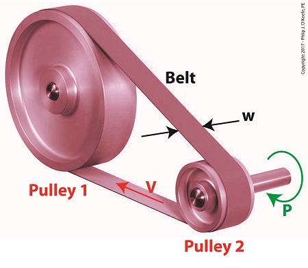
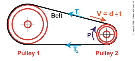
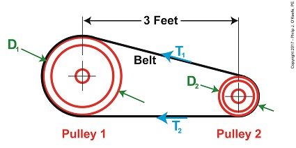
   It’s been awhile since we began our discussion of a pulley-belt assembly operating within a hydroponics plant, and we’ve solved for a lot variables and derived many equations along the way.   Today we’ll tackle the two remaining variables,  T1 , the belt’s tight side tension, and T2 , its loose side tension, and we’ll determine exactly what belt width will optimize power transmission within our system.

 Optimizing Belt Width in a Pulley-Belt Assembly

Optimizing Belt Width in a Pulley-Belt Assembly


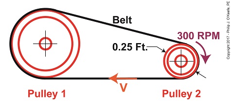
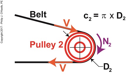
   Last time we converted mechanical power, P, from horsepower into foot-pounds per second and the belt’s velocity, V, into feet per second in order to get things into terms we can work with.   We then inserted these values into the mechanical power formula to get,

2,200 foot pounds per second = (T1 – T2) × 3.93 feet/second               (1)

   This equation will allow us to solve for T1 and T2, and from there we’ll develop a value for the optimum belt width.

   Previously, we determined from the Euler-Eytelwein Formula that,

T1 = 2.38T2                                                                                     (2)

   Substituting equation (2) into equation (1), we get,

2,200 foot pounds per second = (2.38T2  – T2) × 3.93 feet/second      (3)

   Reducing this equation with algebra we arrive at,

T2 = 405.65 pounds                                                                         (4)

   We can now insert equation (4) into equation (2) and calculate T1,

T1 = 2.38 × 405.65 pounds                                                               (5)

T1 = 965.44 pounds                                                                         (6)


   T1 is maximum tension in the belt, specified by the manufacturer to be 300 pounds per inch of width, which makes the minimum width belt to be used to optimize power transmission within our  pulley-belt assembly,

w = T1 ÷ 300 pounds per inch                                                           (7)

w = 965.44 pounds ÷ 300 pounds per inch                                         (8)

w = 3.22 inches                                                                                (9)

   We can use a belt of minimum width of 3.22 inches to safely transmit 4 horsepower from the engine to the pump without incurring breakage and slippage along the belt, thereby optimizing power transmission within our assembly.   If we used a narrower belt, breaking and slippage would occur.   If we used a wider belt, an unnecessary expense would be incurred.

   Next time we’ll begin a discussion on flywheels as they apply to rotating machinery like gasoline and steam engines.


Copyright 2017 – Philip J. O’Keefe, PE

Engineering Expert Witness Blog

____________________________________


Unit Conversion, Horsepower to Foot-Pounds per Second

Monday, September 4th, 2017

   We’ve been working our way towards developing values for variables in our example pulley-belt assembly, and last time we calculated the velocity of the belt in that assembly to be 237.99 feet per minute.   But before we can go on to calculate the belt’s loose side tension, T2, and tight side tension, T1, we’ll need to discuss unit conversion, specifically how to convert horsepower into foot-pounds per second.

   Our working formula for this demonstration is the formula for mechanical power, P, previously introduced and shown again here,

P = (T1 – T2) × V                                                               (1)

   By engineering convention mechanical power is normally measured in units of foot-pounds per second.   But if you’ll recall from a past blog in which we determined the belt’s velocity, V, it was measured in units of feet per minute, not per second. 

   To further complicate things, the difference in belt tensions, T1 – T2, is stated in units of pounds, and combining these elements together results in P being expressed in foot-pounds per minute, not the required per second, because we are multiplying feet per minute by pounds.   That’s a whole lot of unit changing within a single equation, which makes for an awkward situation.

   To smooth things out we’ll have to do some converting of units.   We’ll start by dividing V by 60 seconds per minute so it can be expressed in units of feet per second,

V = 237.99 feet per minute ÷  60 seconds per minute          (2)

 V = 3.93 feet/second                                                        (3)

   The power in our belt was previously given as 4 horsepower, which must also undergo conversion and be put in terms of foot-pounds per second so it can be used in equation (1).

Unit Conversion, Horsepower into Foot-Pounds

Unit Conversion, Horsepower to Foot-Pounds per Second


   One horsepower is equal to 550 foot-pounds per second, which makes the amount of power, P, in our pulley-belt assembly equal to 2,200 foot-pounds per second.

   Units converted, we can now insert the values for V and P into equation (1) to arrive at,

2,200 foot pounds per second = (T1 – T2) × 3.93 feet/second           (4)

   Next time we’ll use this relationship to develop values for T1 and T2, the belt’s tight and loose side tensions.

Copyright 2017 – Philip J. O’Keefe, PE

Engineering Expert Witness Blog

____________________________________


Belt Velocity

Monday, August 21st, 2017

   Last time we developed an equation to compute tangential velocity, V, of the belt in our example pulley and belt system.   Today we’ll plug numbers into this equation and arrive at a numerical value for this belt velocity.

Belt Velocity

Belt Velocity


   The equation we’ll be working with is,

V = π × D2 ÷  t2                                                        (1)

where, D2 is the diameter of Pulley 2 and π represents the constant 3.1416. We learned that Pulley 2’s period of revolution, t2, is related to its rotational speed, N2, which represents the time it takes for it to make one revolution and is represented by this equation,

N2 = 1 ÷ t2                                                                            (2)

   We’ll now solve for the belt’s velocity, V, using known values, starting off with rearranging terms so we can solve for t2,

t2 = 1 ÷ N                                                                         (3)

   We were previously given that N2 is 300 RPM, or revolutions per minute, so equation (3) becomes,

t2 = 1 ÷ 300 RPM = 0.0033 minutes                         (4)

   This tells us that Pulley 2 takes 0.0033 minutes to make one revolution in our pulley-belt assembly.

   Pulley 2’s diameter, D2, was previously determined to be 0.25 feet.    Inserting this value equation (1) becomes,

 V = π × (0.25 feet) ÷ (0.0033 minutes)                  (5)

 V = 237.99 feet/minute                                         (6)


   We’ve now determined that the belt in our pulley-belt assembly zips around at a velocity of 237.99 feet per minute.

   Next time we’ll apply this value to equation (6) and determine the belt’s tight side tension, T1.

Copyright 2017 – Philip J. O’Keefe, PE

Engineering Expert Witness Blog

____________________________________


Tangential Velocity

Monday, August 14th, 2017

   Last time we introduced the Mechanical Power Formula, which is used to compute power in pulley-belt assemblies, and we got as far as introducing the term tangential velocity, V, a key variable within the Formula.   Today we’ll devise a new formula to compute this tangential velocity.

   Our starting point is the formula introduced last week to compute the amount of power, P, in our pulley-belt example is, again,

P = (T1 – T2) × V                                         (1)

   We already know that P is equal to 4 horsepower, we have yet to determine the belt’s tight side tension, T1, and loose side tension, T2, and of course V, the formula for which we’ll develop today.


Tangential Velocity

Tangential Velocity


   Tangential velocity is dependent on both the circumference, c2, and rotational speed, N2, of Pulley 2.  The circumference represents the length of Pulley 2’s curved surface.   The belt travels part of this distance as it makes its way from Pulley 2 back to Pulley 1. The rotational speed, N2, represents the rate that it takes for Pulley 2’s curved surface to make one revolution while propelling the belt.   This time period is known as the period of revolution, t2, and is related to N2 by this equation,

N2 = 1 ÷ t2                                                                         (2)

   The rotational speed of Pulley 2 is specified in our example as 300 RPMs, or revolutions per minute, and we’ll denote that speed as N2 in light of the fact it’s referring to speed present at the location of Pulley 2.   As we build the formula, we’ll be converting N2 into velocity, specifically tangential velocity, V, which is the velocity at which the belt operates, this in turn will enable us to solve equation (1).

   Why speak in terms of tangential velocity rather than plain old ordinary velocity?  Because the moving belt’s orientation to the surface of the pulley lies at a tangent in relation to the pulley’s circumference, c2, as shown in the above illustration.   Put another way, the belt enters and leaves the curved surface of the pulley in a straight line.

   Generally speaking, velocity is distance traveled over a period of time, and tangential velocity is no different.  So taking time into account we arrive at this formula,

V = c2 ÷ t2                                                                          (3)

   Since the surface of Pulley 2 is a circle, its circumference can be computed using a formula developed thousands of years ago by the Greek engineer and mathematician Archimedes.   It is,

c2 = π × D2                                                            (4)

where D2 is the diameter of the pulley and π represents the constant 3.1416.

   We now arrive at the formula for tangential velocity by combining equations (3) and (4),

V = π × D2 ÷ t2                                                    (5)

   Next time we’ll plug numbers into equation (5) and solve for V.

Copyright 2017 – Philip J. O’Keefe, PE

Engineering Expert Witness Blog

____________________________________


The Mechanical Power Formula in Pulley and Belt Assemblies

Saturday, July 29th, 2017

     Last time we determined the value for one of the key variables in the Euler-Eytelwein Formula known as the angle of wrap.   To do so we worked with the relationship between the two tensions present in our example pulley-belt assembly, T1 and T2.   Today we’ll use physics to solve for T2 and arrive at the Mechanical Power Formula, which enables us to compute the amount of power present in our pulley and belt assembly, a common engineering task.

    To start things off let’s reintroduce the equation which defines the relationship between our two tensions, the Euler-Eytelwein Formula, with the value for e, Euler’s Number, and its accompanying coefficients, as determined from our last blog,

T1 = 2.38T2                            (1)

    Before we can calculate T1 we must calculate T2.   But before we can do that we need to discuss the concept of power.

 The Mechanical Power Formula in Pulley and Belt Assemblies

 The Mechanical Power Formula in Pulley and Belt Assemblies


    Generally speaking, power, P, is equal to work, W, performed per unit of time, t, and can be defined mathematically as,

P = W ÷ t                               (2)

    Now let’s make equation (2) specific to our situation by converting terms into those which apply to a pulley and belt assembly.   As we discussed in a past blog, work is equal to force, F, applied over a distance, d.   Looking at things that way equation (2) becomes,

P = F × d ÷ t                         (3)

    In equation (3) distance divided by time, or “d ÷ t,” equals velocity, V.   Velocity is the distance traveled in a given time period, and this fact is directly applicable to our example, which happens to be measured in units of feet per second.   Using these facts equation (3) becomes,

P = F × V                               (4)

    Equation (4) contains variables that will enable us to determine the amount of mechanical power, P, being transmitted in our pulley and belt assembly.

   The force, F, is what does the work of transmitting mechanical power from the driving pulley, pulley 2, to the passive driven pulley, pulley1.   The belt portion passing through pulley 1 is loose but then tightens as it moves through pulley 2.   The force, F, is the difference between the belt’s tight side tension, T1, and loose side tension, T2.   Which brings us to our next equation, put in terms of these two tensions,

P = (T1 – T2) × V                   (5)

    Equation (5) is known as the Mechanical Power Formula in pulley and belt assemblies.

    The variable V, is the velocity of the belt as it moves across the face of pulley 2, and it’s computed by yet another formula.   We’ll pick up with that issue next time.


Copyright 2017 – Philip J. O’Keefe, PE

Engineering Expert Witness Blog

____________________________________


Determining Angle of Wrap

Monday, July 17th, 2017

   Sometimes things which appear simple turn out to be rather complex.   Such is the case with the Euler-Eytelwein Formula, a small formula with a big job.   It computes how friction, an omnipresent phenomenon in mechanical assemblies, contributes to the transmission of mechanical power.   Today we’ll determine the value of one of the Euler-Eytelwein Formula’s variables, the angle of wrap.

Determining Angle of Wrap

Determining Angle of Wrap

   Here again is the basis for our calculations, the Euler-Eytelwein Formula.

T1 = T2 × eθ)                                                                 (1)

   To recap what we’ve discussed thus far, T1 is the tight side tension, the maximum the belt can endure before breaking.   T2 is the loose side tension.   It’s just going along for the ride.   The term e is Euler’s Number, a constant equal to 2.718, and the coefficient of friction, μ, for contact points between the belt and pulleys is 0.3 based on their materials.

   The formula introduced last time to calculate the angle of wrap, θ, is,

θ = (1802α) × (π  ÷ 180)                                             (2)

where,

α = sin-1((D1 – D2) ÷ 2x)                                                 (3)

   By direct measurement we’ve determined the pulleys’ diameters, D1 and D2, are equal to 1 foot and 0.25 feet respectively.   The term x is the distance between the two pulley shafts, 3 feet.   The term sin-1 is a trigonometric function known as inverse sine, a button commonly found on scientific calculators.

   Inserting our known values into equation (3) we arrive at,

α = sin-1((1.0 foot – 0.25 feet) ÷ 2 × (3 feet))                  (4)

α = 7.18                                                                        (5)

   We can now incorporate equation (5) into equation (2) to solve for θ,

θ = (180(2 × 7.18)) × (π ÷ 180)                                  (6)

θ = 2.89                                                                         (7)

   Inserting the values for m and θ into equation (1) we arrive at,

T1 = T2 × 2.718(0.3 × 2.89)                                               (8)

T1 = 2.38T2                                                                    (9)

   We have at this point solved for over half of the unknown variables in the Euler-Eytelwein Formula.   We still can’t solve for T1, because we don’t know the value of T2.   But that will change next time when we introduce yet another formula, this one to determine the amount of mechanical power present in our pulley-belt system.


Copyright 2017 – Philip J. O’Keefe, PE

Engineering Expert Witness Blog

____________________________________