|
We’ve been discussing various aspects of a power plant’s water-to-steam cycle, from machinery specifics to identifying inefficiencies, and today we’ll do more of the same by introducing the condenser hot well and discussing its importance as a key contributor to the conservation of energy, specifically heat energy. Let’s start by returning our attention to the steam inside the condenser vessel. Last week we traced the path of the condenser’s tubes and learned that the cool water contained within them serve to regulate the steam’s temperature surrounding them so that temperatures don’t rise dangerously high. To fully understand the important result of this dynamic we have to revisit the concept of latent heat energy explored in a previous article. More specifically, how this energy factors into the transformation of water into steam and vice versa. Steam entering the condenser from the steam turbine contains latent heat energy that was added earlier in the water/steam cycle by the boiler. This steam enters the condenser just above the boiling point of water, and it will give up all of its latent heat energy due to its attraction to the cool water inside the condenser tubes. This initiates the process of condensation, and water droplets form on the exterior surfaces of the tubes.
The water droplets fall like rain from the tube surfaces into the hot well situated at the bottom of the condenser. This hot well is essentially a large basin that serves as a collection point for the condensed water, otherwise known as condensate. It’s important to collect the condensate in the hot well and not just empty it back into the lake, because condensate is water that has already undergone the process of purification. It’s been made to pass through a water treatment plant prior to being put to use in the boiler, and that purified water took both time and energy to create. The purified condensate also contains a lot of sensible heat energy which was added by the boiler to raise the water temperature to boiling point, as we learned in another previous article. This heat energy was produced by the burning of expensive fuels, such as coal, oil, or natural gas. So it’s clear that the condensate collecting in the hot well has already had a lot of energy put into it, energy we don’t want to lose, and that’s why its an integral part of the water-to-steam setup. It acts as a reservoir, and the drain in its bottom allows the condensate to flow from the condenser, then follow a path to the boiler, where it will be recycled and put to renewed use within the power plant. Next week we’ll follow that path to see how the condensate’s residual heat energy is put to good use. ________________________________________ |
Posts Tagged ‘mechanical engineer’
How A Power Plant Condenser Works, Part 3
Monday, October 14th, 2013
Condensation Inside the Steam Turbine
Sunday, September 8th, 2013|
Did you know that water droplets traveling at high velocity can take on the force of bullets? It can happen, particularly within steam turbines at a power plant during the process of condensation, where steam transforms back into water. The last couple of weeks in this blog series we’ve been talking about the steam and water cycle within electric utility power plants, how heat energy is added to water during the boiling process, and how turbines run on the sensible heat energy that lies within the superheated steam vapor supplied by boilers and superheaters. We learned that without a superheater there is a very real possibility that the steam’s temperature can fall to mere boiling point. When steam returns to boiling point temperature an undesirable situation is created. The steam begins to condense into water within the turbine. To understand how this happens, let’s return to our graph from last week. It illustrates the situation when there’s no superheater present in the power plant’s steam cycle.
Figure 1
After consuming all the sensible heat energy in phase C in Figure 1, the only heat energy which remains available to the turbine is the latent heat energy in phase B. If you recall from past blog articles, latent heat energy is the energy added to the boiler water to initiate the building of steam. As the turbine consumes this final source of heat energy, the steam begins a process of condensation while it flows through the turbine. You can think of condensing as a process that is opposite to boiling. During condensation, steam changes back into water as latent heat energy is consumed by the turbine. When the condensing process is in progress, the temperature in phase B remains at boiling point, but instead of pure steam flowing through the turbine, the steam will now include water droplets, a dangerous mixture. As steam flows through the progressive chambers of turbine blades, more of its latent heat energy is consumed and increasingly more steam turns back into water as the number of water droplets increases.
Figure 2 – Water Droplets Forming in the Turbine
The danger comes in when you consider that the steam/water droplet mixture is flying through the turbine at hundreds of miles per hour. At these high speeds water droplets take on the force of machine gun bullets. That’s because they act more like a solid than a liquid due to their incompressible state. In other words, under great pressure and at high speed water droplets don’t just harmlessly splash around. They hit hard and cause damage to rapidly spinning turbine blades. Without a working turbine, the generator will grind to a halt. So how do we supply the energy hungry turbine with the energy contained within high temperature superheated steam in sufficient quantities to keep things going? We’ll talk more about the superheater, its function and construction, next week.
________________________________________ |


Superheating, Part 2
Sunday, August 25th, 2013|
Last time we added a piece of equipment called a superheater, positioned between the boiler and steam turbine, to our basic electric utility power plant steam and water cycle. Its addition enables a greater and more consistent supply of heat energy to the steam which powers the turbine. How much more? Let’s look at Figure 1 to get an idea.
Figure 1
You may have noticed that our illustration lacks numerical representation. That’s because power plants are designed differently, depending on fuels used and power output required. So unless we’re talking about a particular power plant, number values would be impractical. For example, I could specify a boiling point of 596°F at 1,500 pounds per square inch (PSI), and a superheater outlet temperature of 1,050°F at 1,200PSI, and I could make note of esoteric things like enthalpy (British Thermal Units per pound mass) values on the Heat Energy axis. But to facilitate our discussion we’ll keep things simple and focus on the general process. Figure 1 shows in phase D the additional heat energy being added to the steam, thanks to the superheater. This is significantly more than had been added by the boiler alone, as represented by phase C. The turbine consumes heat energy added in phases C and D and converts it into mechanical energy to drive the generator, resulting in electrical energy being provided to consumers in the most energy efficient way possible. But increasing power output and efficiency isn’t the superheater’s only job. The heat it adds during phase D ensures the turbine’s safe operation when it’s cranking at full capacity, as represented by the superheated steam zones of phases C and D. Next week we’ll discover how the superheater prevents a destructive process known as condensing from occurring inside the turbine. ________________________________________ |

Patent Drawings – “Ordinary Skill in the Art”
Sunday, June 9th, 2013|
Last week I introduced this illustration as a typical patent drawing and asked if you could decipher the riddle of its functionality.
Patent drawings are static, two dimensional (2D) representations of proposed inventions which are meant to be manufactured in three dimensions (3D). As such they present a lot of complex information on a flat page. If you don’t have a clue as to what this machine is, I guarantee you’re not alone. The average person wouldn’t. There’s a bunch of lines, shapes and numbers, but what do they signify? How are they meant to all come together and operate? As a matter of fact, the average person isn’t meant to understand patent drawings. That’s because they’re not what patent courts have defined as a person of ordinary skill in the art, a peculiar term which basically means that the Average Joe or Josephine isn’t meant to be able to interpret them. Rather, the interpretation of patent drawings is left to individuals with specialized skills and training, a particular educational background and/or work experience. These individuals are typically able to view a static 2D image and visualize how the illustrated device moves, how it operates. Those said to fall within the court’s definition as having ordinary skill in the art are in fact often engineers and scientists. Since the average person does not have a background in engineering and science, it can be challenging for patent attorneys to present their cases in the courtroom, particularly when relying on 2D representations alone. That’s where animations come in. Next time we’ll use the magic of animation to transform our cryptic 2D patent illustration into a functional 3D animation of a machine whose operation is easily understood by the average person. ___________________________________________ |

Patent Drawings
Sunday, June 2nd, 2013|
I remember the first time I saw a blueprint. It was during high school shop class where we learned how to use power tools to make the wooden chairs, tables, and chests shown in blueprints. I was completely confused. The odd paper and blue print, coupled with the liberal use of unfamiliar symbols, dashes and dots, and what appeared to be a mind boggling amount of detail was enough to start me in a cold sweat. For many people, patent drawings are a lot like that first blueprint I saw. As a static two-dimensional (2D) representation of an operational device which is often complex, they present an immense amount of information on a page. The average person would be hard pressed to interpret them, and in fact, as we’ll learn later, they aren’t supposed to be able to. We’ve been talking about patent basics in this series of blogs, and we’ll continue that discussion in the following weeks with a concentration on patent drawings. In the meantime, here’s one to ponder. When you look at a patent drawing like the one below, what do you see? What do you think this thing is and what is it supposed to do? We’ll find out next week…
___________________________________________ |
Determining Patent Eligibility – Part 3, What Constitutes a Machine?
Sunday, April 21st, 2013|
One of my favorite toys as a kid was Mr. Machine. He was a windup mechanical man that swung his arms when he walked while repeatedly squawking a strange YAK! sound. His body was transparent, so all the gears and levers inside were visible, and he even came with his own repair wrench. Alas, his wrench was of little use when Mr. Machine took a tragic fall down the basement stairs. Mr. Machine was aptly named. There’s no question but that he was a machine, because his inventor received a US patent, No. 3,050,900. In order to accomplish this he had to have met guidelines set out in federal statutes, specifically those contained in 35 USC § 101. He had to prove that Mr. Machine was a bona fide machine.
If you’ll recall from last week’s discussion, in order to secure a patent, inventions must prove to be original technology that is classifiable as a machine, an article of manufacture, a composition of matter, or a process, or an improvement upon same. Last week our focus was on utility, the first hurdle that an invention must jump for it to be patent eligible. Let’s continue our discussion on patentability by examining the second hurtle. When you consider the word machine, you might imagine something containing mechanical parts, like my childhood mechanical friend. But in the world of patents that’s not necessarily the case. There, a machine can be mechanical, electrical, electronic, or electromechanical in nature. In other words, a machine can include anything from a cell phone to a rocket. To be precise, under patent law the definition of machine includes any physical device consisting of two or more parts which dynamically interact with each other. For example, a purely mechanical machine, such as a diesel engine, has many moving parts. Those parts, the pistons, connecting rods, etc., are mechanically linked to dynamically interact, or move together, when the engine runs. Next week we’ll consider less obvious examples of what constitutes a machine under patent law. ___________________________________________ |


Strength of Materials – Poisson’s Ratio
Sunday, January 16th, 2011| Rubber bands, plastic food wrap, bandages that conform to knuckles and knees, where would we be without them? These are all fairly recent inventions, but their elastic properties were imagined far before they actually came into existence.
Around the turn of the 19th Century a mathematics genius by the name of Siméon Denis Poisson dabbled in higher level mathematics. He enjoyed working with calculus and probability theories and their applications, and his work eventually led to the discovery of his own special ratio, the “Poisson ratio.” Denoted today by the Greek letter “µ,” his discovery has a great deal to do with elasticity. In fact, much of his work evolved to become the modern study of engineering. If you’ll remember from last week’s blog, we talked about the elasticity of materials, including materials you generally wouldn’t think of as being elastic. In our steel rod example we saw that when you pull on the ends of a steel rod hard enough, you can actually stretch it and make it longer. But where does this extra length come from? According to Poisson’s ratio, as the rod lengthens, its diameter decreases proportionately. The rod’s increased length comes at the expense of its diameter. You can see this effect at work by repeatedly stretching that fat rubber band whose task it is to contain your bulging Sunday paper. The more you pull on it, the skinnier the rubber band becomes. It will eventually get to the point were its elastic properties have been so compromised it won’t even be able to hold together Monday’s paper. Over the decades that have passed since Poisson’s discovery a multitude of laboratory tests have been conducted to determine µ for a vast number of materials. These values have been duly tabulated in engineering reference books, doing away with the tedious task of conducting individualized experimentation by present day design engineers. Steel, for example, has a Poisson’s ratio of around 0.28, and this number is readily available in most strength of materials reference books. It’s pretty obvious why Poisson’s contribution is important to the world of engineering, but now let’s see how his ratio can be applied. Last week we saw that a 15-foot long, 2-inch diameter round steel rod stretches by 0.115 inches when it is pulled by a steady 60,000 pound force. Poisson’s ratio tell us that this results in an accompanying decrease in diameter, but by how much? To find out, we simply multiply the stretched length of the rod by Poisson’s ratio for steel (µ = 0.28). Plugging these numbers into an equation we see that the diameter decreases by: 0.115 inches × 0.28 = 0.032 inches This is approximately the thickness of nine sheets of paper. So if the rod was 2 inches in diameter before the 60,000 pound force was applied, its new diameter after application of the stretching force would be: 2 inches – 0.032 inches = 1.968 inches The change of .032 in the rod’s diameter may not seem like much, but in the world of machine parts it could mean the difference between parts fitting properly or becoming loose. This wraps up our short series on strengths of elastic materials. Next time we’ll move on to discuss coal power plant fundamentals, an arena in which many of the things we’ve been discussing take on real world meaning. _____________________________________________
|

Diesel Locomotive Brakes
Sunday, June 6th, 2010|
In the past few weeks we’ve taken a look at both mechanical and dynamic brakes. Now it’s time to bring the two together for unparalleled stopping performance. Have you ever wandered along a railroad track, hopping from tie to tie, daring a train to come roaring along and wondering if you could jump to safety in time? Many have, and many have lost the bet. That’s because a train, once set into motion, is one of the hardest things on Earth to bring to a stop. In this discussion, let’s focus on the locomotive. A large, six-axle variety is shown in Figure 1.
Figure 1 – A Six-Axle Diesel-Electric Locomotive These massive iron horses are known in the industry as diesel-electric locomotives, and here’s why. As Figure 2 shows, diesel-electric locomotives are powered by huge diesel engines. Their engine spins an electrical generator which effectively converts mechanical energy into electrical energy. That electrical energy is then sent from the generator through wires to electric traction motors which are in turn connected to the locomotive’s wheels by a series of gears. In the case of a six-axle locomotive, there are six traction motors all working together to make the locomotive move. So how do you get this beast to stop? Figure 2 – The Propulsion System In A Six-Axle Diesel-Electric Locomotive You probably noticed in Figure 2 that there are resistor grids and cooling fans. As long as you’re powering a locomotive’s traction motors to move a train, these grids and fans won’t come into play. It’s when you want to stop the train that they become important. That’s when the locomotive’s controls will act to disconnect the traction motor wires running from the electrical generator and reconnect them to the resistor grids as shown in Figure 3 below.
Figure 3 – The Dynamic Braking System In A Six-Axle Diesel Electric Locomotive The traction motors now become generators in a dynamic braking system. These motors take on the properties of a generator, converting the moving train’s mechanical, or kinetic, energy into electrical. The electrical energy is then moved by wires to the resistor grids where it is converted to heat energy. This heat energy is removed by powerful cooling fans and released into the atmosphere. In the process the train is robbed of its kinetic energy, causing it to slow down. Now you may be thinking that dynamic brakes do all the work, and this is pretty much true, up to a point. Although dynamic brakes may be extremely effective in slowing a fast-moving train, they become increasingly ineffective as the train’s speed decreases. That’s because as speed decreases, the traction motors spin more slowly, and they convert less kinetic energy into electrical energy. In fact, below speeds of about 10 miles per hour dynamic brakes are essentially useless. It is at this point that the mechanical braking system comes into play to bring the train to a complete stop. Let’s see how this switch from dynamic to mechanical dominance takes place. A basic mechanical braking system for locomotive wheels is shown in Figure 4. This system, also known as a pneumatic braking system, is powered by compressed air that is produced by the locomotive’s air pump. A similar system is used in the train’s railcars, employing hoses to move the compressed air from the locomotive to each car.
Figure 4 – Locomotive Pneumatic Braking System In the locomotive pneumatic braking system, pressurized air enters an air cylinder. Once inside, the air bears against a spring-loaded piston, as shown in Figure 4(a). The piston moves, causing brake rods to pivot and clamp the brake shoes to the locomotive’s wheel with great force, slowing the locomotive. When you want to get the locomotive moving again, you vent the air out of the cylinder as shown in Figure 4(b). This takes the pressure off the piston, releasing the force from the brake shoes. The spring in the cylinder is now free to move the shoes away from the wheel so they can turn freely. We have now returned to the situation present in Figure 2, and the locomotive starts moving again. Next week we’ll talk about regenerative braking, a variation on the dynamic braking concept used in railway vehicles like electric locomotives and subway trains. _____________________________________________
|


Dynamic Brakes
Monday, May 31st, 2010|
Last week we looked at how a mechanical brake stopped a rotating wheel by converting its mechanical energy, namely kinetic energy, into heat energy. This week, we’ll see how a dynamic brake works. Chances are you have directly benefited by a dynamic braking system the last time you rode in an elevator. But, to understand the basic principle behind an elevator’s dynamic brake system, let’s first take a look at the electric braking system in Figure 1 below.
Figure 1 – A Simple Electric Braking System Here the brake consists of an electric generator wired via an open switch to an electrical component called a resistor. The weight is attached to a cable that is wound around a pulley on the generator’s shaft. As the weight freefalls, the cable unwinds on the pulley, causing the pulley to turn the generator’s shaft. Unlike last week’s mechanical brake which required a good deal of effort to employ, a dynamic braking system requires very little. All that needs to be done is to close a switch as shown in Figure 2 below. When the switch is closed, an electrical circuit is created where the resistor gets connected to the generator. The resistor does as its name implies: it resists (but doesn’t stop) the electrical current flowing through it from the generator. As the electrical current fights its way through the resistor to get back to the generator, the resistor gets hot like an electric heater. This heat is dissipated to the cooler surrounding air. At the same time, the weight begins to slow down in its descent. But how is this happening? The electric braking system can be thought of as an energy conversion process. We start out with the kinetic, or motion energy, of the freefalling weight. This kinetic energy is transmitted to the electrical generator by the cable, which spins the generator’s shaft as the cable unwinds. Electrical generators are machines that convert kinetic energy into electrical energy. This energy travels from the electric generator through wires and a closed switch to the resistor. In the process the resistor converts the electrical energy into heat energy. So, kinetic energy is drawn from the falling weight through the conversion process and leaves the process in the form of heat. As the falling weight is drained of kinetic energy, it slows down.
Figure 2 – Applying the Electric Brake Okay, now let’s get back to dynamic brakes on elevators. An elevator is attached by a cable to a hoist that is powered by an electric motor. When it’s time to stop at the desired floor, the automatic control system disconnects the elevator’s electric motor from its power source and turns the motor into a generator. The generator is then automatically connected to a resistor like the one shown in the electric brake above. The kinetic energy of the moving elevator is converted by the generator into electrical energy. The resistor converts the electrical energy into heat energy which is then dissipated into the surrounding environment. The elevator slows down in the process because it’s being robbed of kinetic energy. When the dynamic brake slows the elevator down enough, a mechanical brake is introduced, taking over to bring the elevator to a complete stop. This two-fold process serves to reduce wear and tear on the mechanical brake’s parts, lengthening the operational lifespan of the system as a whole. Next time, we’ll tie everything together and show how mechanical and dynamic brakes work together in a diesel locomotive. _____________________________________________
|


A Pump By Any Other Name…
Monday, May 10th, 2010|
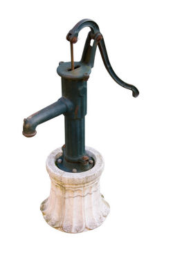
Pumps are all around us. They keep our drinking water flowing, the cooling water circulating in your car’s engine, and even your blood flowing. They’re essential in many aspects of our lives, but most of us don’t think too much about them. For our discussion let’s put them into two categories: positive displacement pumps and centrifugal pumps. This week, we’ll focus on positive displacement pumps. Positive displacement pumps, as their name implies, displace a quantity of liquid with each complete cycle of movement. This takes place when moving parts of the pump take “bites” out of the liquid at the inlet, then force them to exit through the outlet. A familiar example of a positive displacement pump is the type of hand operated water pump that’s commonly found in campgrounds. See Figure 1. Figure 1 – A Positive Displacement Pump This type of pump is known as a reciprocating positive displacement pump. By reciprocating, I mean that the moving parts travel back and forth in a straight line during its operation. Let’s see how it works by referring to the cutaway view in Figure 2. Figure 2 – Cutaway View of the Pump Shown in Figure 1 In the cutaway view, the pump’s piston and internal check valve are shown, and there’s another check valve in the bottom of the pump housing. When you pull up on the handle, the piston moves down into the water in the pump housing, and the pressure caused by this movement forces the check valve in the bottom to slam closed, while the check valve above is forced open. This causes water movement to flood through the open check valve and fill up the space above the piston. When you push down on the handle, the opposite happens. The piston is made to move upward. The upward acceleration of the water above the piston causes the check valve on the piston to slam shut, and this traps the water above it. As the piston moves back up, a suction is created below, which causes the check valve in the bottom of the housing to pop open and more water is drawn up into the space below the piston. Eventually, when the piston gets high enough, the water trapped on top of it will flow out of the spigot. Another type of positive displacement pump is represented by a rotary pump. These pumps operate in a circular motion to move a volume of liquid with each revolution of the pump shaft. This is done by trapping liquid between moving parts, such as gears, lobes, vanes, or screws, and the stationary pump housing itself. To show how this works, refer to the gear pump shown in Figure 3. Its gear teeth mesh together in the middle of the pump, blocking the flow from going straight through and trapping it within the spaces formed by rotating gear teeth and the pump housing. It’s like the water is being forced through a turnstile.
Figure 3 – A Cutaway View of a Gear Pump Next week, we’ll talk about centrifugal pumps and how they move liquids along using centrifugal force.
_____________________________________________
|


