Posts Tagged ‘coefficient of friction’
Monday, July 17th, 2017
|
Sometimes things which appear simple turn out to be rather complex. Such is the case with the Euler-Eytelwein Formula, a small formula with a big job. It computes how friction, an omnipresent phenomenon in mechanical assemblies, contributes to the transmission of mechanical power. Today we’ll determine the value of one of the Euler-Eytelwein Formula’s variables, the angle of wrap.
Determining Angle of Wrap
Here again is the basis for our calculations, the Euler-Eytelwein Formula.
T1 = T2 × e(μθ) (1)
To recap what we’ve discussed thus far, T1 is the tight side tension, the maximum the belt can endure before breaking. T2 is the loose side tension. It’s just going along for the ride. The term e is Euler’s Number, a constant equal to 2.718, and the coefficient of friction, μ, for contact points between the belt and pulleys is 0.3 based on their materials.
The formula introduced last time to calculate the angle of wrap, θ, is,
θ = (180 – 2α) × (π ÷ 180) (2)
where,
α = sin-1((D1 – D2) ÷ 2x) (3)
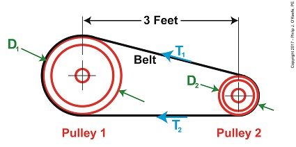
By direct measurement we’ve determined the pulleys’ diameters, D1 and D2, are equal to 1 foot and 0.25 feet respectively. The term x is the distance between the two pulley shafts, 3 feet. The term sin-1 is a trigonometric function known as inverse sine, a button commonly found on scientific calculators.
Inserting our known values into equation (3) we arrive at,
α = sin-1((1.0 foot – 0.25 feet) ÷ 2 × (3 feet)) (4)
α = 7.18 (5)
We can now incorporate equation (5) into equation (2) to solve for θ,
θ = (180 – (2 × 7.18)) × (π ÷ 180) (6)
θ = 2.89 (7)
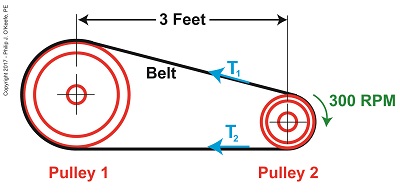
Inserting the values for m and θ into equation (1) we arrive at,
T1 = T2 × 2.718(0.3 × 2.89) (8)
T1 = 2.38T2 (9)
We have at this point solved for over half of the unknown variables in the Euler-Eytelwein Formula. We still can’t solve for T1, because we don’t know the value of T2. But that will change next time when we introduce yet another formula, this one to determine the amount of mechanical power present in our pulley-belt system.
Copyright 2017 – Philip J. O’Keefe, PE
Engineering Expert Witness Blog
____________________________________ |
Tags: angle of wrap, belt, coefficient of friction, Euler-Eytelwein Formula, Euler's Number, friction, loose side tension, mechanical assemblies, mechanical power, pulley, pullies, tight side tension
Posted in Engineering and Science, Expert Witness, Forensic Engineering, Innovation and Intellectual Property, Personal Injury, Product Liability | Comments Off on Determining Angle of Wrap
Wednesday, July 5th, 2017
|
Last time we introduced a scenario involving a hydroponics plant powered by a gas engine and multiple pulleys. Connecting the pulleys is a flat leather belt. Today we’ll take a step further towards determining what width that belt needs to be to maximize power transmission efficiency. We’ll begin by revisiting the two T’s of the Euler-Eytelwein Formula and introducing a formula to determine a key variable, angle of wrap.
The Angle of Wrap Formula
We must start by calculating T1, the tight side tension of the belt, which is the maximum tension the belt is subjected to. We can then calculate the width of the belt using the manufacturer’s specified safe working tension of 300 pounds per inch as a guide. But first we’ll need to calculate some key variables in the Euler-Eytelwein Formula, which is presented here again,
T1 = T2× e(μθ) (1)
We determined last time that the coefficient of friction, μ, between the two interfacing materials of the belt and pulley are, respectively, leather and cast iron, which results in a factor of 0.3.
The other factor shown as a exponent of e is the angle of wrap, θ, and is calculated by the formula,
θ = (180 – 2α) × (π ÷ 180) (2)
You’ll note that this formula contains some unique terms of its own, one of which is familiar, namely π, the other, α, which is less familiar. The unnamed variable α is used as shorthand notation in equation (2), to make it shorter and more manageable. It has no particular significance other than the fact that it is equal to,
α = sin-1((D1 – D2) ÷ 2x) (3)
If we didn’t use this shorthand notation for α, equation (2) would be written as,
θ = (180 – 2(sin-1((D1 – D2) ÷ 2x))) × (π ÷ 180) (3a)
That’s a lot of parentheses!
Next week we’ll get into some trigonometry when we discuss the diameters of the pulleys, which will allow us to solve for the angle of wrap.
Copyright 2017 – Philip J. O’Keefe, PE
Engineering Expert Witness Blog
____________________________________ |
Tags: angle of wrap, belt, belt tension, coefficient of friction, Euler-Eytelwein Formula, mechanical power transmission, pulley, pulleys
Posted in Engineering and Science, Expert Witness, Forensic Engineering, Innovation and Intellectual Property, Personal Injury, Product Liability | Comments Off on The Angle of Wrap Formula
Friday, June 23rd, 2017
|
Belts are important. They make fashion statements, hold things up, keep things together. Today we’re introducing a scenario in which the Euler-Eytelwein Formula will be used to, among other things, determine the ideal width of a belt to be used in a mechanical power transmission system consisting of two pulleys inside a hydroponics plant. The ideal width belt would serve to maximize friction between the belt and pulleys, thus controlling slippage and maximizing belt strength to prevent belt breakage.
An engineer is tasked with designing an irrigation system for a hydroponics plant. Pulley 1 is connected to the shaft of a water pump, while Pulley 2 is connected to the shaft of a small gasoline engine.
What Belt Width does a Hydroponics Plant Need?
Mechanical power is transmitted by the belt from the engine to the pump at a constant rate of 4 horsepower. The belt material is leather, and the two pulleys are made of cast iron. The coefficient of friction, μ, between these two materials is 0.3, according to Marks Standard Handbook for Mechanical Engineers. The belt manufacturer specifies a safe working tension of 300 pounds force per inch width of the belt. This is the maximum tension the belt can safely withstand before breaking.
We’ll use this information to solve for the ideal belt width to be used in our hydroponics application. But first we’re going to have to re-visit the two T’s of the Euler-Eytelwein Formula. We’ll do that next time.
Copyright 2017 – Philip J. O’Keefe, PE
Engineering Expert Witness Blog
____________________________________ |
Tags: belt, belt breakage, coefficient of friction, engine, engineer, horsepower, leather belt, mechanical power transmission, pulley, pump
Posted in Engineering and Science, Expert Witness, Forensic Engineering, Innovation and Intellectual Property, Personal Injury, Product Liability | Comments Off on What Belt Width does a Hydroponics Plant Need?
Tuesday, June 13th, 2017
|
Last week we saw how friction coefficients as used in the Euler-Eyelewein Formula, can be highly specific to a specialized application, U.S. Navy ship capstans. In fact, many diverse industries benefit from aspects of the Euler-Eytelwein Formula. Today we’ll introduce another engineering application of the Formula, exploring its use within the irrigation system of a hydroponics plant.
Another Specialized Application of the Euler-Eyelewein Formula
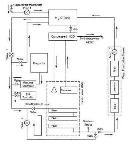
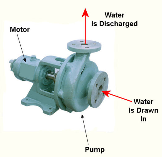
Pumps conveying water are an indispensable part of a hydroponics plant. In the schematic shown here they are portrayed by the symbol ⊗.
In our simplified scenario to be presented next week, these pumps are powered by a mechanical power transmission system, each consisting of two pulleys and a belt. One pulley is connected to a water pump, the other pulley to a gasoline engine. A belts runs between the pulleys to deliver mechanical power from the engine to the pump.
The width of the belts is a key component in an efficiently running hydroponics plant. We’ll see how and why that’s so next time.
Copyright 2017 – Philip J. O’Keefe, PE
Engineering Expert Witness Blog
____________________________________ |
Tags: belt, belt width, coefficient of friction, engineering, Euler-Etytelwein Formula, gasoline engine, hydroponics, mechanical power transmission, power, pulley, pump
Posted in Engineering and Science, Expert Witness, Forensic Engineering, Innovation and Intellectual Property, Personal Injury, Product Liability, Professional Malpractice | Comments Off on Another Specialized Application of the Euler-Eyelewein Formula
Wednesday, April 27th, 2016
|
Last time we introduced the frictional force formula which is used to calculate the force of friction present when two surfaces move against one another, a situation which I as an engineering expert must sometimes negotiate. Today we’ll plug numbers into that formula to calculate the frictional force present in our example scenario involving broken ceramic bits sliding across a concrete floor.
Here again is the formula to calculate the force of friction,
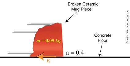
FF = μ × m × g
where the frictional force is denoted as FF, the mass of a piece of ceramic sliding across the floor is m, and g is the gravitational acceleration constant, which is present due to Earth’s gravity. The Greek letter μ, pronounced “mew,” represents the coefficient of friction, a numerical value predetermined by laboratory testing which represents the amount of friction at play between two surfaces making contact, in our case ceramic and concrete.
To calculate the friction present between these two materials, let’s suppose the mass m of a given ceramic piece is 0.09 kilograms, μ is 0.4, and the gravitational acceleration constant, g, is as always equal to 9.8 meters per second squared.
Calculating the Force of Friction
Using these numerical values we calculate the force of friction to be,
FF = μ × m × g
FF = (0.4) × (0.09 kilograms) × (9.8 meters/sec2)
FF = 0.35 kilogram meters/sec2
FF = 0.35 Newtons
The Newton is shortcut notation for kilogram meters per second squared, a metric unit of force. A frictional force of 0.35 Newtons amounts to 0.08 pounds of force, which is approximately equivalent to the combined stationary weight force of eight US quarters resting on a scale.
Next time we’ll combine the frictional force formula with the Work-Energy Theorem formula to calculate how much kinetic energy is contained within a single piece of ceramic skidding across a concrete floor before it’s brought to a stop by friction.
Copyright 2016 – Philip J. O’Keefe, PE
Engineering Expert Witness Blog
____________________________________ |
Tags: coefficient of friction, Earth's gravity, engineering expert, force of friction, friction, frictional force, frictional force formula, gravitational acceleration constant, kinetic energy, Newtons, weight force, work-energy theorem
Posted in Engineering and Science, Expert Witness, Forensic Engineering, Innovation and Intellectual Property, Personal Injury, Product Liability, Professional Malpractice | Comments Off on Calculating the Force of Friction
Thursday, April 14th, 2016
|
Last time we introduced the force of friction, another force in our ongoing discussion about changing forms of energy, and we learned that it’s often a counterproductive force which design engineers and engineering experts such as myself must work to minimize in order to optimize functionality of devices we’re designing. Today we’ll introduce the frictional force formula, which computes the amount of friction present when two surfaces meet.
To demonstrate frictional force, we’ve been working with the example of a shattered mug’s broken ceramic pieces and watching their progress as they slide across a concrete floor. They eventually come to a stop not too far from the point where the mug shattered, because friction causes them to stop. The mass of the ceramic pieces in combination with the downward pull of gravity causes the broken bits to “bear down” on the floor, thereby maximizing contact and creating friction.
At first glance the floor and mugs’ surfaces may appear slippery smooth, but when viewed under magnification we see that both actually contain many peaks and valleys. The peaks of one surface project into the valleys of the other and it’s fight, fight, fight for the ceramic pieces to continue their progress across the floor. The strength of the frictional force acting upon the pieces is a factor of their individual weights coupled with the roughness of the two surfaces coming into contact — the shattered pieces and the floor. If friction didn’t exist and no other impediments were in the way, the pieces might travel to the next state before stopping!
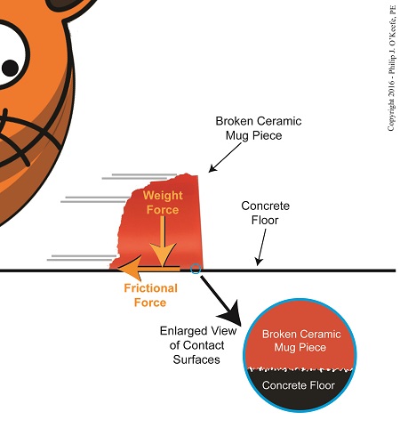
Frictional Force Resists Motion
Last time we introduced Charles-Augustin de Coulomb, a scientist whose work with friction led to the later development of a formula to calculate it. It’s presented here, and frictional force is denoted as FF,
FF = μ × m × g
where, m is the mass of an object making contact with another surface and g is the gravitational acceleration constant, which is due to the force of Earth’s gravity. The Greek letter μ, pronounced “mew,” represents the coefficient of friction, a number. Numerical values for μ were determined by laboratory testing and are recorded in engineering books for many combinations of materials, including rubber on concrete, leather on steel, wood on aluminum, and our own example of ceramic on concrete.
Next time we’ll plug the numbers that apply to our ceramic-on-concrete example into the friction formula and calculate the frictional force at play.
Copyright 2016 – Philip J. O’Keefe, PE
Engineering Expert Witness Blog
____________________________________ |
Tags: Charles-Augustin de Coulomb, coefficient of friction, Earth's gravity, energy, engineering expert, friction, friction force formula, frictional force, gravitational acceleration constant, mass, mu
Posted in Engineering and Science, Expert Witness, Forensic Engineering, Innovation and Intellectual Property, Personal Injury, Product Liability | Comments Off on The Frictional Force Formula
Sunday, May 23rd, 2010
Imagine driving in your car, you’re traveling at a speed of 65 mph and you’re coming up on a curve. You depress your brake pedal to negotiate the turn, and nothing happens…
Scenarios just like this one have been in the news quite often lately, brakes which just aren’t operating correctly. We’ve heard the tales of terror, recounted by those unfortunate individuals who have been placed in this situation, but have we reflected on just why their brakes might have failed?
Put most simply, a brake is a device whose purpose is to stop a body in motion. This important task is accomplished by converting the kinetic energy (energy of motion) into heat energy. This can be accomplished by either of two methods, mechanically or electrically. In today’s blog we’ll focus on the mechanical aspect.
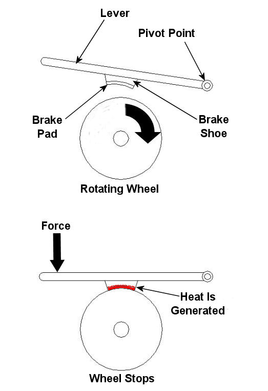
A simple mechanical brake is shown in Figure 1 below. In this arrangement kinetic energy is converted into heat energy when force is applied to a lever, causing a brake shoe to meet up with a rotating wheel. The brake shoe has a pad attached to its surface that makes direct contact with the wheel, and when the two come together great friction is produced. It’s this friction that will ultimately stop the object in motion. Friction turns the kinetic energy into heat energy.

Figure 1 – A Simple Mechanical Brake
Friction at its simplest is a mechanical resistance to movement. Whenever two materials in motion come into contact with each other there is always some degree of friction. The extent to which friction is produced by their meeting is referred to as the “coefficient of friction.”
The coefficient of friction varies according to the surface character of the materials coming in contact. For example, the coefficient of friction for the leather sole of your shoe on smooth ice is very low. This means you’ll do a lot of slipping when you’re trying to walk, and that’s because ice presents little friction to resist a smoothly soled shoe. But take this same shoe and apply it to the rough surface of concrete, and you’ll be walking quickly and efficiently. Coefficients of friction between different materials have been duly measured in laboratories and are tabulated for easy access in engineering reference books.
Based on our simple example above, one would easily come to the conclusion that a high coefficient of friction is desirable when talking about brake shoes, specifically the one represented in Figure 1 above. The higher the coefficient of friction, the more the pad wants to grab the wheel, and the less force you will need to apply to the brake shoe to successfully come to a stop.
That’s mechanical braking in a nutshell. Next time, we’ll focus on an electrical braking system known as a “dynamic brake.”
_____________________________________________

|
Tags: brake pad, brake shoe, brakes, braking systems, coefficient of friction, design engineeringing, engineering expert witness, forensic engineering, heat energy, kinetic energy, mechanical brake
Posted in Engineering and Science, Product Liability | Comments Off on Brakes and Braking Systems


