Posts Tagged ‘forensic engineering’
Thursday, March 24th, 2016
|
Last time we watched our example ceramic coffee mug crash to a concrete floor, where its freefall kinetic energy performed the work of shattering it upon impact. This is a scenario familiar to engineering experts like myself who are sometimes asked to reconstruct accidents and their aftermaths, otherwise known as forensic engineering. Today we’ll take a look at what happens when the shattered mug’s pieces are freed from their formerly cozy, cohesive bond, and we’ll watch their transmutation from kinetic energy to work, and back to kinetic energy.
As we watch our mug shatter on the floor, we notice that it breaks into different sized pieces that are broadcast in many directions around the point of impact. Each piece has its own unique mass, m, travels at its own unique velocity, v, and has a unique and individualized amount of kinetic energy. This is in accordance with the kinetic energy formula, shown here again:
KE = ½ × m × v2
So where did that energy come from?

The Scattering Pieces Have Kinetic Energy
According to the Work-Energy Theorem, the shattered mug’s freefalling kinetic energy is transformed into the work that shatters the mug. Once shattered, that work is transformed back into kinetic energy, the energy that fuels each piece as it skids across the floor.
The pieces spray out from the point of the mug’s impact until they eventually come to rest nearby. They succeed in traveling a fair distance, but eventually their kinetic energy is dissipated due to frictional force which slows and eventually stops them.
The frictional force acting in opposition to the ceramic pieces’ travel is created when the weight of each fragment makes contact with the concrete floor’s rough surface, which creates a bumpy ride. The larger the fragment, the more heavily it bears down on the concrete and the greater the frictional force working against it. With this dynamic at play we see smaller, lighter fragments of broken ceramic cover a greater distance than their heavier counterparts.
The Work-Energy Theorem holds that the kinetic energy of each piece equals the work of the frictional force acting against it to bring it to a stop. We’ll talk more about this frictional force and its impact on the broken pieces’ distance traveled next time.
Copyright 2016 – Philip J. O’Keefe, PE
Engineering Expert Witness Blog
____________________________________ |
Tags: engineering expert, force, forensic engineering, friction force, kinetic energy, kinetic energy formula, mass, velocity, work, work-energy theorem
Posted in Engineering and Science, Expert Witness, Forensic Engineering, Innovation and Intellectual Property, Personal Injury, Product Liability | Comments Off on Kinetic Energy to Work, Work to Kinetic Energy
Monday, June 30th, 2014
|
Last time we set up an example where an electric motor is connected to a lathe via a gear train. Today we’ll take the numerical values present on that gear train and plug them into the torque ratio equation we’ve been working with for the past few blogs.
In the illustration below the electric motor exerts 200 inch pounds of torque upon the driving gear. The driving gear pitch circle diameter is 6 inches, while the driven gear pitch circle diameter is 8 inches. It’s been determined through previous lab testing that the lathe we’ll be using requires at least 275 inch pounds of torque to be exerted upon the driven gear shaft in order to operate properly. Will the gear train shown below meet this requirement?

First, a review of the torque ratio equation:
T1 ÷ T2 = D1 ÷ D2
Now we’ll crunch numbers. T1 is equal to 200 inch pounds, D1 is equal to 3 inches (pitch radius equals pitch diameter divided by two), and D2 is equal to 4 inches. This gives us:
(200 inch pounds) ÷ T2 = (3 inches) ÷ (4 inches)
T2 = (200 inch pounds) ÷ (0.75) = 266.67 inch pounds
So, does the gear train as presented here supply enough torque to power the lathe properly? No, it does not. It provides only 266.67 inch pounds, not the 275 inch pounds of torque required.
Next time we’ll see how to manipulate gear sizes within a gear train in order to meet a given torque requirement.
_______________________________________
|
Tags: driven gear, driving gear, electric motor, engineering expert witness, forensic engineering, gear expert witness, gear pitch, gear train, gear train torque, inch pounds of torque, lathe, mechanical engineering expert witness, mechanism, motor, pitch circle, pitch diameter, torque equations, torque ratio equation
Posted in Engineering and Science, Expert Witness, Forensic Engineering, Innovation and Intellectual Property, Personal Injury, Product Liability | Comments Off on Determining Torque Within a Gear Train
Wednesday, March 26th, 2014
|
Last time we introduced a physics concept known as torque and how it, together with modified gear ratios, can produce a mechanical advantage in devices whose motors utilize gear trains. Now we’ll familiarize ourselves with torque’s mathematical formula, which involves some terminology, symbols, and concepts which you may not be familiar with, among them, vectors, and sin(ϴ).
Torque = Distance × Force × sin(ϴ)
In this formula, Distance and Force are both vectors. Generally speaking, a vector is a quantity that has both a magnitude — that is, any measured quantity associated with a vector, whether that be measured in pounds or inches or any other unit of measurement — and a direction. Vectors are typically represented graphically in engineering and physics illustrations by pointing arrows. The arrows are indicative of the directionality of the magnitudes involved.
Sin(ϴ), pronounced sine thay-tah, is a function found within a field of mathematics known as trigonometry , which concerns itself with the lengths and angles of triangles. ϴ, or thay-tah, is a Greek symbol used to represent the angle present between the Force and Distance vectors as they interact to create torque. The value of sin(ϴ) depends upon the number of degrees in the angle ϴ. Sin(ϴ) can be found by measuring the angle ϴ, entering its value into a scientific calculator, and pressing the Sin button.
We’ll dive into the math behind the vectors next time, when we return to our wrench and nut example and apply vector force quantities.
_______________________________________
|
Tags: direction, distance, engineering, engineering expert witness, force, forensic engineering, gear ratio, gear train, gears, magnitude, physics, sine, theta, torque, trigonometry, vector
Posted in Engineering and Science, Expert Witness, Forensic Engineering, Innovation and Intellectual Property, Personal Injury, Product Liability | Comments Off on Vectors, Sin(ϴ), and the Torque Formula
Monday, November 18th, 2013
|
Last time we learned how enthalpy is used to measure heat energy contained in the steam inside a power plant. The higher the steam pressure, the higher the enthalpy, and vice versa, and we touched upon the concept of work, or the potential for a useful outcome of a process. Today we’ll see how to get the maximum work out of a steam turbine by attaching a condenser at the point of its exhaust and making the most of the vacuum that exists within its condenser.
Let’s revisit the equation introduced last time, which allows us to determine the amount of useful work output:
W = h1 – h2
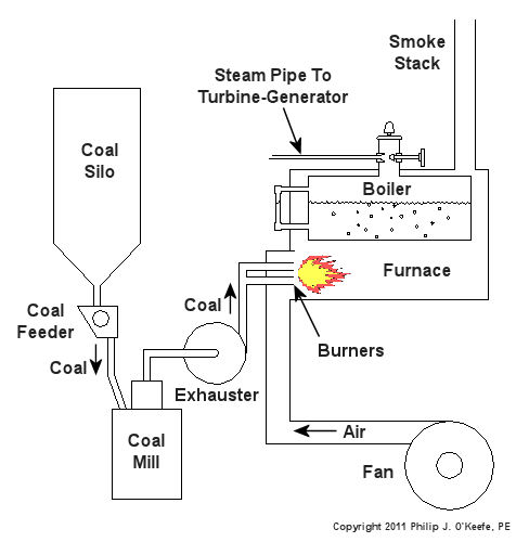
Applied to a power plant’s water-to-steam cycle, enthalpy h1 is solely dependent on the pressure and temperature of steam entering the turbine from the boiler and superheater, as contained within the purple dashed line in the diagram below.

As for enthalpy h2, it’s solely dependent on the pressure and temperature of steam within the condenser portion of the water-to-steam cycle, as shown by the blue dashed circle of the diagram.
Next week we’ll see how the condenser, and more specifically the vacuum inside of it, sets the platform for increased energy production, a/k/a work.
________________________________________
|
Tags: boiler, coal power plant expert witness, condensate, condenser, electric generator, electric utility power plant expert, energy, engineering expert witness, enthalpy, forensic engineering, power engineering expert witness, power plant equipment, power plant training, steam pressure, steam temperature, steam turbine, superheater, turbine exhaust, turbine generator, vacuum, water-to-steam cycle, work
Posted in Engineering and Science, Expert Witness, Forensic Engineering, Innovation and Intellectual Property, Personal Injury, power plant training, Product Liability | Comments Off on Enthalpy and the Potential for More Work
Monday, January 9th, 2012
| It’s a dark and stormy night and you’ve come to the proverbial fork in the road. The plot is about to take a twist as you’re forced to make a decision in this either/or scenario. As we’ll see in this article, an electric relay operates in much the same manner, although choices will be made in a forced mechanical environment, not a cerebral one.
When we discussed basic electric relays last week we talked about their resting in a so-called “normal state,” so designated by industrial control parlance. It’s the state in which no electric current is flowing through its wire coil, the coil being one of the major devices within a relay assembly. Using Figure 3 of my previous article as a general reference, in this normal state a relaxed spring keeps the armature touching the N.C. switch contact. While in this state, a continuous conductive path is created for electricity through to the N.C. point. It originates from the wire on the left side, which leads to the armature pivot point, travels through the armature and N.C. contact points, and finally dispenses through the wire at the right leading from the N.C. contact.
Now let’s look at an alternate scenario, when current is made to flow through the coil. See Figure l, below.

Figure 1
Figure 1 shows the path of electric current as it flows through the wire coil, causing the coil and the steel core to which it’s attached to become magnetized. This magnetization is strong, attracting the steel armature and pulling it towards the steel core, thus overcoming the spring’s tension and its natural tendency to rest in a tension-free state.
The magnetic attraction causes the armature to rotate about the pivot point until it comes to rest against the N.O. contact, thus creating an electrical path en route to the N.O. wire, on its way to whatever device it’s meant to energize. As long as current flows through the wire coil, its electromagnetic nature will attract the armature to it and contact will be maintained with the N.O. juncture.
When current is made to flow through the wire coil, an air gap is created between the armature and the N.C. contact, and this prevents the flow of electric current through the N.C. contact area. Current is forced to follow the path to the N.O. contact only, effectively cutting off any other choice or fork in the road as to electrical path that may be followed. We can see that the main task of an electric relay is to switch current between two possible paths within a circuit, thereby directing its flow to one or the other.
Next time we’ll examine a simple industrial control system and see how an electric relay can be engaged with the help of a pushbutton.
____________________________________________ |
Tags: armature, coil, control relay, control system, current flow, electric current, electric relay, electrical path, electrical relay, electrical switch, electricity, electromagnetic, engineering expert witness, forensic engineering, industrial control, magnetic attraction, N.C., N.C. contact, N.O., N.O. contact, normal state, normally closed, normally open, pushbutton, relay, relay ladder logic, spring, steel core, switch, switch contact, switching current, wire coil
Posted in Engineering and Science, Expert Witness, Forensic Engineering, Innovation and Intellectual Property, Personal Injury, Product Liability, Professional Malpractice | 1 Comment »
Sunday, September 25th, 2011
| Ever wonder why the burger you get at your favorite fast food chain never looks like the one on TV? The bun isn’t fluffy, the beef patty doesn’t make it to the edges, and the lettuce is anything but crisp. Well, it’s because a professional known as a Food Stylist, working together with a professional marketing firm and production crew, has painstakingly created the beautiful, bright and balanced burger used to lure you in. The process can take days or even weeks to create and has nothing to do with reality. The burger you’re really going to get will look more like a gorilla sat on it.
Many of the same issues must be dealt with when mass producing food. Chances are human hands will never even touch the product, like they did when creating the prototype in the test kitchen. In the world of food manufacturing, the “look” part can be extremely challenging. How do you get machines and production lines to create visually appealing food that entices prospective buyers to make an investment in it? How do you get it to taste good, or at least acceptable to the palate?
The “taste” part of food manufacturing can be even more challenging. For example, in the test kitchen of a pastry product manufacturer, a recipe will be developed using home pantry products like flour, butter, and eggs. Ever made bread or a pie crust? The stickiness factor is enough to drive many insane. Even nimble human fingers have a hard time dealing with it. Now enter food processing machinery and conveyor belts into the scenario. This brings the possibility of stickiness to a whole new level. Huge messes that gum up the machinery are common, and production line shutdowns are the result.
When faced with these challenges, plant engineers have to work closely with chefs in the R&D kitchen to come up with some sort of compromise in the recipe or final form of the food product. The goal is to cost effectively produce food products acceptable to consumers for purchase, and it’s often an iterative process involving many successive changes to recipes and equipment designs, coupled with a lot of testing and retesting, before success is finally met. If testing ultimately proves that the product appeals to consumers’ tastes and flows nicely through production lines, then there’s a good chance it will be a commercial success. In any case, cost is the dictating factor as to whether the food product will successfully make it onto the shelves of your supermarket. A margin of profit must be made.
But this success is only part of the design process. Before full commercial production can commence, processing equipment and production lines must be designed so that they:
- Are easy to clean at the end of the production run.
- Don’t contaminate the food during operation.
- Are easy to operate and maintain.
- Can be easily modified to make other products.
Next time we’ll explore how cleanliness requirements factor into food manufacturing equipment design.
____________________________________________

|
Tags: cleanliness, contamination, conveyor belt, engineering expert witness, food equipment design, food manufacturing, food processing machinery, food production, forensic engineering, machines, maintenance, plant engineer
Posted in Engineering and Science | Comments Off on Food Manufacturing Challenges – Look and Taste
Sunday, July 31st, 2011
| The evolution of cooking methods has been interesting indeed, from the open fires of primitive man, who must have decided at some point that cooked meat tasted better than raw, on to wood fired stoves, fossil fuel-based cooking, whether coal, propane, or gas, and let’s not forget electric range tops. Standing on its own in the modern kitchen is the microwave oven. What will be next? The space age food pill dispensing stations of the futuristic cartoon family, The Jetsons?
We’ve been talking about resonant cavity magnetrons and the purpose they serve within a microwave radar system. We also learned about Dr. Percy Spencer’s discovery and how microwave radar transmissions emanating from a magnetron can cook food, not to mention melt candy bars.

Figure 1- Microwaves Melt Candy Bars and Cook Food
Although the technologies used in microwave radars and microwave ovens are similar, they do have important differences. It would be both unsafe and impractical to install microwave radar systems into kitchens. Radiation emitted from radar wave guide lacking proper containment would bounce aimlessly around the kitchen, posing a threat to human safety. You see, microwaves don’t know the difference between our bodies and the food we wish to cook. They’ll heat up human tissue just as readily as a bowl of chicken soup. Another issue is that runaway microwaves lose much of their effectiveness through their aimless bouncing about, and much of it would not be directed to the food itself. Dr. Spencer would learn how to corral that energy, making microwave cooking a commercial success.
The biggest problem for Dr. Spencer to overcome was containment of the microwaves. They needed to be directed towards food in order to efficiently heat them. His first microwave oven was a metal box containing an opening at the top into which a magnetron wave guide could be inserted. This would then introduce microwaves into the box, and the metal construction of the box would safely contain them. The safety issue had now been resolved because the waves couldn’t escape, they would simply bounce around inside the box and most of their energy would be transferred into any food placed inside.
Dr. Spencer’s employer, the Raytheon Corporation, produced the first commercial microwave oven in 1954, and it was appropriately named the “Radarange.” It was huge, almost six feet tall, and weighed in at about 750 pounds! Hardly something that could fit into a home kitchen. Despite its massive size, the Radarange wasn’t all that powerful and couldn’t compete against the compact countertop microwave ovens in use today.
It wasn’t until 1967 that technology improved enough to give us the smaller, more efficient units affordable to consumers. This improvement involved using a newly developed semiconductor device called a “diode” within the high voltage electric circuitry that powers the magnetron. We’ll learn more about these technologies in our next post.
Also in our next post, we’ll see how high voltage circuits can pose electrocution hazards in a way you‘d never expect. I discussed one of these instances in my recent appearance on The Discovery Channel program, Curious and Unusual Deaths, soon to be aired.
_____________________________________________ |
Tags: coal, curious and unusual deaths, diode, Discovery Channel, electric range, electrocution, engineering expert witness, forensic engineering, gas, high voltage circuit, magnetron, microwave oven, microwave radar, microwave radiation, propane, radar transmission, resonant cavity magentron, semiconductor, stove, wave guide
Posted in Engineering and Science, Expert Witness, Forensic Engineering, Innovation and Intellectual Property, Personal Injury, Product Liability | Comments Off on The Microwave Oven Becomes Reality
Sunday, February 27th, 2011
|
We’ve been talking about coal fired power plants for some time now, and it’s always good to introduce third party information on subject matter in order to gain the most from the discussion. What follows is an excerpt of an interesting book review on the subject of coal consumption which appeared in the New York Times:
There is perhaps no greater act of denial in modern life than sticking a plug into an electric outlet. No thinking person can eat a hamburger without knowing it was once a cow, or drink water from the tap without recognizing, at least dimly, that its journey began in some distant reservoir. Electricity is different. Fully sanitized of any hint of its origins, it pours out of the socket almost like magic.
In his new book, Jeff Goodell breaks the spell with a single number: 20. That’s how many pounds of coal each person in the United States consumes, on average, every day to keep the electricity flowing. Despite its outdated image, coal generates half of our electricity, far more than any other source. Demand keeps rising, thanks in part to our appetite for new electronic gadgets and appliances; with nuclear power on hold and natural gas supplies tightening, coal’s importance is only going to increase. As Goodell puts it, “our shiny white iPod economy is propped up by dirty black rocks.”
To read the entire article, follow this link:
http://www.nytimes.com/2006/06/25/books/review/25powell.html?_r=2

A locomotive crane unloading coal from railcars at a power plant in the late 1930s.
Next week we’ll continue our regular series, following energy’s journey through the power plant.
_____________________________________________ |
Tags: coal, coal consumption, coal power plant fundamentals, coal power plant training, electric utility engineer, electric utility training, electricity generation, engineering expert witness, forensic engineering, fossil fuel, heat energy, locomotive crane, power cycle, power engineering, power industry, railcars
Posted in Engineering and Science, Expert Witness, Forensic Engineering, Personal Injury, power plant training, Professional Malpractice | 1 Comment »
Sunday, February 20th, 2011
|
When I was a kid I didn’t have video games or cable TV to help me occupy my time. Back then parents tended to be frugal, and the few games I had were cheap to buy and simple in operation, like the plastic toy windmill I’d play with for hours on end. All I had to do to make it spin was take a deep breath, pucker my lips together, fill my cheeks with breath, then blow hard into the windmill blades. Its spin was fascinating to watch. Little did I know that as an adult I would come to work with a much larger and complex version of it, in the form of a power plant’s steam turbine.
You see, when you trap breath within bulging cheeks and then squeeze your cheek muscles together, you actually create a pressurized environment. This air pressure buildup transfers energy from your mouth muscles into the trapped breath within your mouth, so that when you open your lips to release the breath through your puckered lips, the pressurized energy is converted into kinetic energy, a/k/a the energy of movement. The breath molecules flow at high speed from your lips to the toy windmill’s blades, and as they come into contact with the blades their energy is transferred to them, causing the blades to move. A similar process takes place in the coal power plant, where steam from a boiler takes the place of pressurized breath and a steam turbine takes the place of the toy windmill.
If you recall from my previous article, the heat energy released by burning coal is transferred to water in the boiler, turning it to steam. This steam leaves the boiler under great pressure, causing it to travel through pipe to the steam turbine, as shown in Figure 1.

Figure 1 – A Basic Steam Turbine and Generator In A Coal Fired Power Plant
At its most basic level the inside of a steam turbine looks much like our toy windmill, of course on a much larger scale, and it is very appropriately called a “wheel.” See Figure 2.

Figure 2 – A Very Basic Steam Turbine Wheel
The wheel is mounted on a shaft and has numerous blades. It makes use of the pressurized steam that has made its way to it from the boiler. This steam has ultimately passed through a nozzle in the turbine that is directed towards the blades on the wheel. This is the point at which heat energy in the steam is converted into kinetic energy. The steam shoots out of the nozzle at high speed, coming into contact with the blades and transferring energy to them, which causes the turbine shaft to spin. The turbine shaft is connected to a generator, so the generator spins as well. Finally, the spinning generator converts the mechanical energy from the turbine into electrical energy.
In actuality, most coal power plant steam turbines have more than one wheel and there are many nozzles. The blades are also more numerous and complex in shape in order to maximize the energy transfer from the steam to the wheels. My Coal Power Plant Fundamentals seminar goes into far greater detail on this and other aspects of steam turbines, but what I have shared with you above will give you a basic understanding of how they operate.
So to sum it all up, the steam turbine’s job is to convert the heat energy of steam into mechanical energy capable of spinning the electrical generator. Next time we’ll see how the generator works to complete the last step in the energy conversion process, that is, conversion of mechanical energy into electrical energy.
_____________________________________________ |
Tags: boiler, coal power plant training, electric utility training, electrical generator, engineering expet witness, forensic engineering, fossil fuel, generating station, heat energy, high pressure steam, kinetic energy, nozzle, power engineering, pressure, seminar, steam, steam pipe, steam turbine, turbine blade, turbine generator, windmill
Posted in Engineering and Science, Personal Injury, power plant training | 5 Comments »
Sunday, November 14th, 2010
|
How many crickets clicking their legs together in unison would it take before we would suffer hearing loss at the sound exposure? Would we need to sit in a garden filled with millions of them all night long, only to discover in the morning that we could no longer hear the tea kettle’s whistle? The chart below may not provide the answer to this question, but it does provide some very good examples of different sounds and the point at which they become hazardous.
So how do we know where we’re at safety-wise with sound pressure levels and exposure times? This question wasn’t pondered until the 1950s, when the military, specifically the Air Force, provided the first standards in this regard in 1956. This initial action was followed up by numerous studies and standards committees wrestling with the issue. It wasn’t until 1981 that the Occupational Health and Safety Administration (OSHA) required employers to implement hearing conservation programs for employees in certain noise-filled environments.
What surprised many of the first scientists studying the impact of sound is that sounds don’t necessarily have to be initially perceived as “too loud” in order to cause hearing loss. Many sounds that we perceive as easily tolerated can in fact cause hearing damage if exposure is long enough.
So what’s “long enough?” Title 29 of the Code of Federal Regulations, Section 1910.95, lists the OSHA permissible sound exposure durations at various sound levels, as shown in Table 1.
|
| Duration of Exposure (Hrs.) |
Sound Level (dB) |
| 8 |
90 |
| 6 |
92 |
| 4 |
95 |
| 3 |
97 |
| 2 |
100 |
| 1.5 |
102 |
| 1 |
105 |
| 0.5 |
110 |
| 0.25 or less |
115 |
Table 1 – OSHA Permissible Noise Exposures
|
Just to put things into perspective, a small chain saw tearing into a log typically produces sound at 90dB, or 90 decibels, which you will recall from last week’s article is the measuring unit used for sound. And that noisy truck clattering down your street, the one that your dog can’t help but bark at, can produce 100dB. The guy standing on the airport tarmac directing your plane into the gate can be exposed to as much as 150dB. There’s a good reason he’s wearing ear protection.
Let’s take a closer look at the information provided in Table 1. It states that you most likely will not suffer hearing loss if you spend up to 8 hours in a place where the sound level does not exceed 90dB. Comparing that information to Table 2, which is specific to noises produced at a power plant, we see that this sound level is produced by the typical steam turbine.
One thing to keep in mind is that when we are exposed to various sounds throughout the day, we can compute a time-weighted average noise, or TWAN, to help us determine if our overall environment poses a threat to our hearing. This method of assessing the gross impact of many different sound exposures is represented by the formula:
TWAN = (C1 ÷ T1) + (C2 ÷ T2) + (C3 ÷ T3) + …
where C represents the total time of exposure at a measured sound level, and T represents the total time of exposure. T, which in our example stands for “hours,” is found in the left column of Table 1. Based on scientific studies of sound’s effects on the human ear, if the TWAN is greater than 1.0, then the exposure exceeds safe limits.
Let’s find out if a worker in a coal fired power plant is at risk of losing his hearing during the course of a typical eight hour workday. Table 2 shows the different noises he has to contend with during that time.
|
| Duration of Exposure (Hrs.) |
Location |
Sound Level (dB) |
| 0.5 |
Steam Turbine Basement |
90 |
| 2.5 |
Air Compressor Room |
95 |
| 0.25 |
Forced Draft Fan Gallery |
110 |
Table 2 – Example Exposure in an 8 Hour Day
|
Now let’s find out if his OSHA recommended sound exposure limit has been exceeded. The values for C, or total time of exposure, are given in the left column, and the corresponding sound level in dB’s is shown in the right column of Table 2. Using these numbers as a reference, we now correlate them with the information contained in Table 1 which cites the OSHA standards. Plugging in the numbers, we find that this worker’s TWAN would be:
TWAN = (0.5 hours ÷ 8 hours) + (2.5 hours ÷ 4 hours) + (0.25 hours ÷ 0.5 hours)
= 1.18
Since 1.18 is greater than 1.0, we see that the worker’s noise limit would indeed be exceeded. He would need to either wear hearing protection or limit his exposure time in order to comply with OSHA regulations and protect his hearing.
Next time we’ll discuss options open to us to control sounds in our environment.
_____________________________________________
|
Tags: air compressor, chain saw, dB, decibels, engineering expert witness, FD fan, forensic engineering, hearing damage, hearing loss, hearing protection, jet engine, loudness, noise, noise control, OSHA, power plant, sound, sound exposure, sound exposure standards, sound level measurement, steam turbine, time weighted average noise, TWAN
Posted in Engineering and Science, Personal Injury, Product Liability | Comments Off on Sound and Exposure Standards


