Archive for the ‘Professional Malpractice’ Category
Monday, July 23rd, 2018
|
So far in this series of articles, we have talked about pneumatic actuators that move jelly filling through a depositor on a pastry production line in a food manufacturing plant. These actuators have pistons with piston rods that create linear motion. The direction of this motion depends on which side compressed air is admitted to the piston inside the actuator. Now, let’s begin discussing a device known to engineers as a solenoid valve. These valves are used to selectively admit compressed air to either side of the pneumatic actuator’s piston, and thus, change the direction of the actuator’s linear motion.
As a solenoid valve’s name implies, a key component is a solenoid. A solenoid consists of a tube, having a coil of wire wrapped around its exterior. Electrical wires extend from the coil to an electrical switch and a voltage supply of, for example, 120 Volts. Inside the tube, there is a steel plunger that is free to move. When the switch is open, the coil is de-energized. That is, no electric current flows from the voltage supply through the coil of wire.
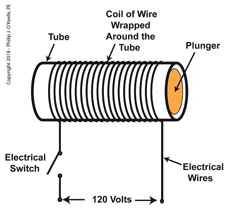
A De-Energized Solenoid
When the electrical switch is closed, the coil becomes energized. As electrical current flows through the coil, a magnetic field is created in the tube. This field forces the steel plunger out of the tube. The magnetic field and force on the plunger remain as long as the switch is closed.
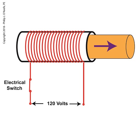
An Energized Solenoid
A solenoid valve consists of a solenoid that is attached to a metal valve body. The solenoid is typically enclosed in a plastic or metal housing. The valve body contains various ports. The ports are threaded holes for the connection of compressed air pipes.
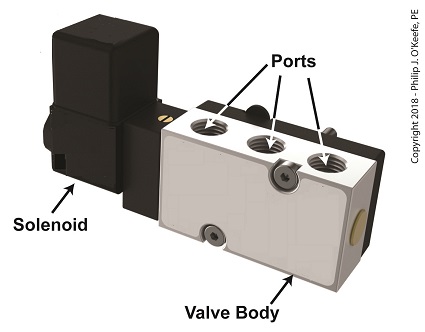
A Solenoid Valve
The solenoid’s plunger is attached to spool in the valve body. The spool is free to move within the valve body past passage ways extending from the ports. In the following illustration, the solenoid valve contains five ports, designated A through E.
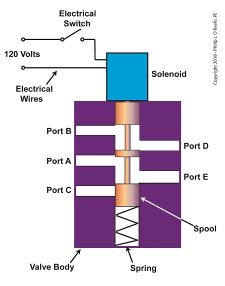
The Solenoid Valve’s Components
Next time we’ll see how the five port solenoid valve operates to create different compressed air flow paths between its ports.
Copyright 2018 – Philip J. O’Keefe, PE
Engineering Expert Witness Blog
____________________________________ |
Tags: coil, compressed air, depositor, engineers, food manufacturing, jelly filling, magnetic field, pastry line, plunger, port, solenoid, solenoid valve, spool, switch, valve body, voltage source
Posted in Engineering and Science, Expert Witness, Forensic Engineering, Innovation and Intellectual Property, Personal Injury, Product Liability, Professional Malpractice | Comments Off on The Solenoid Valve’s Components
Monday, May 7th, 2018
|
Last time we learned that the risk of damaging cavitation bubbles forming at a centrifugal pump’s inlet can be eliminated by simply increasing the water level inside the tank. Today we’ll do the math that demonstrates how reducing cavitation can be accomplished by raising tank elevation.

Reducing Cavitation by Raising Tank Elevation–Before
In our example we’ll suppose that we’re having a problem with cavitation bubbles forming at the inlet, where water temperature is 108ºF and water level inside the tank stands at 33 inches. We are using the formula,
P = γ × h (1)
Equation (1) was introduced previously to correlate water pressure, P, with the specific weight of water, (0.036 pounds/inch3), and the height, h, of the water surface in the tank. If h is 33 inches, then we obtain,
P = (0.036 pounds/inch3) × (33 inches) = 1.2 pounds/inch2 (2)
So, the weight of the water in the tank exerts a pressure of 1.2 pounds per square inch (PSI) at the bottom of the tank and the pump inlet when it sits at the same elevation as the tank.
We know that if we increase the water depth in the tank relative to the pump inlet, we can raise the pressure at the pump inlet in accordance with equation (1). Raising the pressure will eliminate the cavitation bubbles that can form there. But, our tank is of fixed volume, and we can’t add more water to raise water depth beyond 33 inches. However, we can increase the elevation of the tank with respect to the inlet, which will produce the same effect. We’ll use equation (1) to determine the tank elevation, h, that will provide the needed increase.
Referring to the thermodynamic properties of water as found in tables appearing in engineering texts, we determine that if we keep water temperature at 108ºF but raise the pressure at the pump inlet from 1.2 PSI to 1.5 PSI, while maintaining current water depth in the tank, cavitation will cease. In other words, we need to increase P by 0.3 PSI.
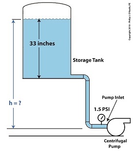
Example of Reducing Cavitation by Tank Elevation–After
Plugging our known values into equation (1) we solve for h,
0.3 PSI = 0.036 pounds/inch3 × h (3)
h = 0.3 PSI ÷ 0.036 pounds/inch3 (4)
h = 8.3 inches (5)
Cavitation will cease when we elevate the tank by 8.3 inches with respect to the pump.
Yet another means of increasing inlet pressure is to install a booster pump. We’ll talk about that next time.
Copyright 2018 – Philip J. O’Keefe, PE
Engineering Expert Witness Blog
____________________________________
|
Tags: cavitation, centrifugal pump, engineering, pump inlet, specific weight of water, stopping cavitation, thermodynamics, water depth, water pressure, water tank elevation
Posted in Engineering and Science, Expert Witness, Forensic Engineering, Innovation and Intellectual Property, power plant training, Product Liability, Professional Malpractice | Comments Off on Reducing Cavitation by Raising Tank Elevation
Thursday, October 26th, 2017
|
Last time we introduced the fact that spinning flywheels are subject to both linear and angular velocities, along with a formula that allows us to calculate these quantities for a single part of the flywheel, designated A. We also re-visited the kinetic energy formula. Today we’ll build upon those formulas as we attempt to answer the question, How much kinetic energy is contained within a spinning flywheel?
Here again is the basic kinetic energy formula,
KE = ½ × m × v2 (1)
where, m equals a moving object’s mass and v is its linear velocity.
Here again is the formula used to calculate linear and angular velocities for a single part A within the flywheel, where part A’s linear velocity is designated vA, angular velocity by ω, and where rA is the distance of part A from the flywheel’s center of rotation.
vA = rA × ω (2)
Working with these two formulas, we’ll insert equation (2) into equation (1) to obtain a kinetic energy formula which allows us to calculate the amount of energy contained in part A of the flywheel,
KEA = ½ × mA × (rA × ω)2 (3)
which simplifies to,
KEA = ½ × mA × rA2 × ω2 (4)
Equation (4) is a great place to begin to calculate the amount of kinetic energy contained within a spinning flywheel, however it is just a beginning, because a flywheel contains many parts. Each of those parts has its own mass, m, and is a unique distance, r, from the flywheel’s center of rotation, and all these parts must be accounted for in order to arrive at a calculation for the total amount of kinetic energy contained within a spinning flywheel.
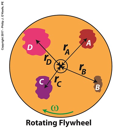
How Much Kinetic Energy is Contained Within a Spinning Flywheel?
Put another way, we must add together all the m × r2 terms for each and every part of the entire flywheel. How many parts are we speaking of? Well, that depends on the type of flywheel. We’ll discuss that in detail later, after we define a phenomenon that influences the kinetic energy of a flywheel known as the moment of inertia.
For now, let’s just consider the flywheel’s parts in general terms. A general formula to compute the kinetic energy contained within the totality of a spinning flywheel is,
KE = ½ × ∑[m × r2] × ω2 (5)
We’ll discuss the significance of each of these variables next time when we arrive at a method to calculate the kinetic energy contained within all the many parts of a spinning flywheel
.
Copyright 2017 – Philip J. O’Keefe, PE
Engineering Expert Witness Blog
____________________________________ |
Tags: angular velocity, center of rotation, engineering, flywheel, kinetic energy, linear velocity, mass, moment of inertia
Posted in Engineering and Science, Expert Witness, Forensic Engineering, Innovation and Intellectual Property, Personal Injury, Product Liability, Professional Malpractice | Comments Off on How Much Kinetic Energy is Contained Within a Spinning Flywheel?
Thursday, October 19th, 2017
|
Anyone who has spun a potter’s wheel is appreciative of the smooth motion of the flywheel upon which they form their clay, for without it the bowl they’re forming would display irregularities such as unattractive bumps. The flywheel’s smooth action comes as a result of kinetic energy, the energy of motion, stored within it. We’ll take another step towards examining this phenomenon today when we take our first look at calculating this kinetic energy. To do so we’ll make reference to the two types of velocity associated with a spinning flywheel, angular velocity and linear velocity, both of which engineers must negotiate anytime they deal with rotating objects.
Let’s begin by referring back to the formula for calculating kinetic energy, KE. This formula applies to all objects moving in a linear fashion, that is to say, traveling a straight path. Here it is again,
KE = ½ × m × v2
where m is the moving object’s mass and v its linear velocity.
Flywheels rotate about a fixed point rather than move in a straight line, but determining the amount of kinetic energy stored within a spinning flywheel involves an examination of both its angular velocity and linear velocity. In fact, the amount of kinetic energy stored within it depends on how fast it rotates.
For our example we’ll consider a spinning flywheel, which is basically a solid disc. For our illustrative purposes we’ll divide this disc into hypothetical parts, each having a mass m located a distance r from the flywheel’s center of rotation. We’ll select a single part to examine and call that A.
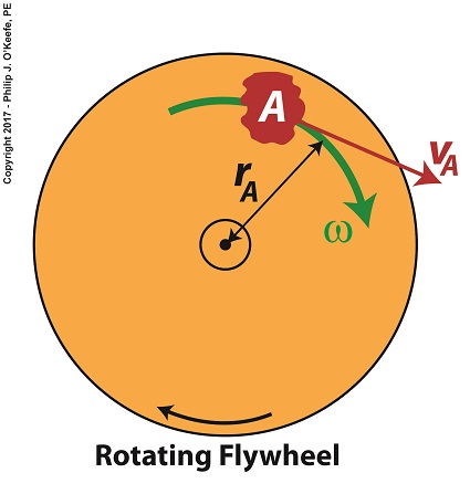
Two Types of Velocity Associated With a Spinning Flywheel
Part A has a mass, mA, and is located a distance rA from the flywheel’s center of rotation. As the flywheel spins, part A rides along with it at an angular velocity, ω, following a circular path, shown in green. It also moves at a linear velocity, vA, shown in red. vA represents the linear velocity of part A measured at any point tangent to its circular path. This linear velocity would become evident if part A were to become disengaged from the flywheel and cast into the air, whereupon its trajectory would follow a straight line tangent to its circular path.
The linear and angular velocities of part A are related by the formula,
vA = rA × ω
Next time we’ll use this equation to modify the basic kinetic energy formula so that it’s placed into terms that relate to a flywheel’s angular velocity. This will allow us to define a phenomenon at play in the flywheel’s rotation, known as the moment of inertia.
Copyright 2017 – Philip J. O’Keefe, PE
Engineering Expert Witness Blog
____________________________________ |
Tags: angular velocity, energy stored, engineering, flywheel, kinetic energy, linear velocity, mass, moment of inertia, spinning flywheel
Posted in Engineering and Science, Expert Witness, Forensic Engineering, Innovation and Intellectual Property, Personal Injury, Product Liability, Professional Malpractice | Comments Off on Two Types of Velocity Associated With a Spinning Flywheel
Tuesday, June 13th, 2017
|
Last week we saw how friction coefficients as used in the Euler-Eyelewein Formula, can be highly specific to a specialized application, U.S. Navy ship capstans. In fact, many diverse industries benefit from aspects of the Euler-Eytelwein Formula. Today we’ll introduce another engineering application of the Formula, exploring its use within the irrigation system of a hydroponics plant.
Another Specialized Application of the Euler-Eyelewein Formula
Pumps conveying water are an indispensable part of a hydroponics plant. In the schematic shown here they are portrayed by the symbol ⊗.
In our simplified scenario to be presented next week, these pumps are powered by a mechanical power transmission system, each consisting of two pulleys and a belt. One pulley is connected to a water pump, the other pulley to a gasoline engine. A belts runs between the pulleys to deliver mechanical power from the engine to the pump.
The width of the belts is a key component in an efficiently running hydroponics plant. We’ll see how and why that’s so next time.
Copyright 2017 – Philip J. O’Keefe, PE
Engineering Expert Witness Blog
____________________________________ |
Tags: belt, belt width, coefficient of friction, engineering, Euler-Etytelwein Formula, gasoline engine, hydroponics, mechanical power transmission, power, pulley, pump
Posted in Engineering and Science, Expert Witness, Forensic Engineering, Innovation and Intellectual Property, Personal Injury, Product Liability, Professional Malpractice | Comments Off on Another Specialized Application of the Euler-Eyelewein Formula
Saturday, January 7th, 2017
|
Last time we saw how the presence of friction reduces mechanical advantage in an engineering scenario utilizing a compound pulley. We also learned that the actual amount of effort, or force, required to lift an object is a combination of the portion of the force which is hampered by friction and an idealized scenario which is friction-free. Today we’ll begin our exploration into how friction results in reduced work input, manifested as heat energy lost to the environment. The net result is that work input does not equal work output and some of Mr. Toga’s labor is unproductive.
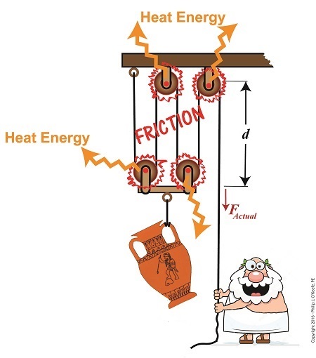
Friction Results in Heat and Lost Work Within a Compound Pulley
In a past blog, we showed how the actual force required to lift our urn is a combination of F, an ideal friction-free work effort by Mr. Toga, and FF , the extra force he must exert to overcome friction present in the wheels,
FActual = F + FF (1)
Mr. Toga is clearly working to lift his turn, and generally speaking his work effort, WI, is defined as the force he employs multiplied by the length, d, of rope that he pulls out of the compound pulley during lifting. Mathematically that is,
WI = FActual × d (2)
To see what happens when friction enters the picture, we’ll first substitute equation (1) into equation (2) to get WI in terms of F and FF,
WI = (F + FF ) × d (3)
Multiplying through by d, equation (3) becomes,
WI = (F × d )+ (FF × d) (4)
In equation (4) WI is divided into two terms. Next time we’ll see how one of these terms is beneficial to our lifting scenario, while the other is not.
Copyright 2017 – Philip J. O’Keefe, PE
Engineering Expert Witness Blog
____________________________________ |
Tags: compound pulley, engineering, friction, heat energy, lost work, mechanical advantage, pulley, reduced work, work input, work output
Posted in Engineering and Science, Expert Witness, Forensic Engineering, Innovation and Intellectual Property, Personal Injury, Product Liability, Professional Malpractice | Comments Off on Friction Results in Heat and Lost Work Within a Compound Pulley
Monday, December 19th, 2016
Tags: engineering expert, engineering expert witness, pulleys
Posted in Courtroom Visual Aids, Engineering and Science, Expert Witness, Forensic Engineering, Innovation and Intellectual Property, Personal Injury, power plant training, Product Liability, Professional Malpractice | Comments Off on Pulleys Make Santa’s Job Easier
Friday, November 18th, 2016
|
We’re all familiar with the phrase, “too much of a good thing.” As a professional engineer, I’ve often found this to be true. No matter the subject involved, there inevitably comes a point when undesirable tradeoffs occur. We’ll begin our look at this phenomenon in relation to compound pulleys today, and we’ll see how the pulley arrangement we’ve been working with encounters a rope length tradeoff. Today’s arrangement has a lot of pulleys lifting an urn a short distance.
We’ll be working with two distance/length factors and observe what happens when the number of pulleys is increased. Last time we saw how the compound pulley is essentially a work input-output device, which makes use of distance factors. In our example below, the first distance/length factor, d1, pertains to the distance the urn is lifted above the ground. The second factor, d2, pertains to the length of rope Mr. Toga extracts from the pulley while actively lifting. It’s obvious that some tradeoff has occurred just by looking at the two lengths of rope in the image below as compared to last week. What we’ll see down the road is that this also affects mechanical advantage.
The compound pulley here consists of 16 pulleys, therefore it provides a mechanical advantage, MA, of 16. For a refresher on how MA is determined, see our preceding blog.
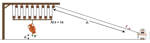
Rope Length Tradeoff in a Compound Pulley
With an MA of 16 and the urn’s weight, W, at 40 pounds, we compute the force, F, Mr. Toga must exert to actively lift the urn higher must be greater than,
F > W ÷ MA
F > 40 Lbs. ÷ 16
F > 2.5 Lbs.
Although the force required to lift the urn is a small fraction of the urn’s weight, Mr. Toga must work with a long and unwieldy length of rope. How long? We’ll find out next time when we’ll take a closer look at the relationship between d1 and d2.
Copyright 2016 – Philip J. O’Keefe, PE
Engineering Expert Witness Blog
____________________________________ |
Tags: compound pulley, effor, force, mechanical advantage, professional engineer, pulley, rope length, weight force, work
Posted in Courtroom Visual Aids, Engineering and Science, Forensic Engineering, Innovation and Intellectual Property, Personal Injury, Product Liability, Professional Malpractice | Comments Off on Rope Length Tradeoff in a Compound Pulley
Thursday, October 27th, 2016
|
Last time we saw how compound pulleys within a dynamic lifting scenario result in increased mechanical advantage to the lifter, mechanical advantage being an engineering phenomenon that makes lifting weights easier. Today we’ll see how the mechanical advantage increases when more fixed and movable pulleys are added to the compound pulley arrangement we’ve been working with.
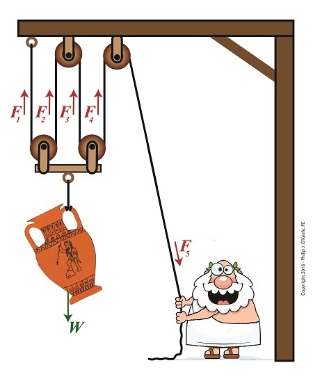
More Pulleys Increase Mechanical Advantage
The image shows a more complex compound pulley than the one we previously worked with. To determine the mechanical advantage of this pulley, we need to determine the force, F5, Mr. Toga exerts to hold up the urn.
The urn is directly supported by four equally spaced rope sections with tension forces F1, F2, F3, and F4. The weight of the urn, W, is distributed equally along the rope, and each section bears one quarter of the load. Mathematically this is represented by,
F1 = F2 = F3 = F4 = W ÷ 4
If the urn’s weight wasn’t distributed equally, the bar directly above it would tilt. This tilting would continue until equilibrium was eventually established, at which point all rope sections would equally support the urn’s weight.
Because the urn’s weight is equally distributed along a single rope that’s threaded through the entire pulley arrangement, the rope rule, as I call it, applies. The rule posits that if we know the tension in one section of rope, we know the tension in all rope sections, including the one Mr. Toga is holding onto. Therefore,
F1 = F2 = F3 = F4 = F5 = W ÷ 4
Stated another way, the force, F5 , Mr. Toga must exert to keep the urn suspended is equal to the weight force supported by each section of rope, or one quarter the total weight of the urn, represented by,
F5 = W ÷ 4
If the urn weighs 40 pounds, Mr. Toga need only exert 10 pounds of bicep force to keep it suspended, and today’s compound pulley provides him with a mechanical advantage, MA, of,
MA = W ÷ F5
MA = W ÷ (W ÷ 4)
MA = 4
It’s clear that adding the two extra pulleys results in a greater benefit to the man doing the lifting, decreasing his former weight bearing load by 50%. If we added even more pulleys, we’d continue to increase his mechanical advantage, and he’d be able to lift far heavier loads with a minimal of effort. Is there any end to this mechanical advantage? No, but there are undesirable tradeoffs. We’ll see that next time.
Copyright 2016 – Philip J. O’Keefe, PE
Engineering Expert Witness Blog
____________________________________ |
Tags: compound pulley, engineering, fixed pulley, lifting, mechanical advantage, movable pulley, rope section, tension force
Posted in Engineering and Science, Forensic Engineering, Innovation and Intellectual Property, Personal Injury, Product Liability, Professional Malpractice | Comments Off on More Pulleys Increase Mechanical Advantage
Wednesday, April 27th, 2016
|
Last time we introduced the frictional force formula which is used to calculate the force of friction present when two surfaces move against one another, a situation which I as an engineering expert must sometimes negotiate. Today we’ll plug numbers into that formula to calculate the frictional force present in our example scenario involving broken ceramic bits sliding across a concrete floor.
Here again is the formula to calculate the force of friction,
FF = μ × m × g
where the frictional force is denoted as FF, the mass of a piece of ceramic sliding across the floor is m, and g is the gravitational acceleration constant, which is present due to Earth’s gravity. The Greek letter μ, pronounced “mew,” represents the coefficient of friction, a numerical value predetermined by laboratory testing which represents the amount of friction at play between two surfaces making contact, in our case ceramic and concrete.
To calculate the friction present between these two materials, let’s suppose the mass m of a given ceramic piece is 0.09 kilograms, μ is 0.4, and the gravitational acceleration constant, g, is as always equal to 9.8 meters per second squared.
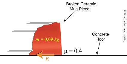
Calculating the Force of Friction
Using these numerical values we calculate the force of friction to be,
FF = μ × m × g
FF = (0.4) × (0.09 kilograms) × (9.8 meters/sec2)
FF = 0.35 kilogram meters/sec2
FF = 0.35 Newtons
The Newton is shortcut notation for kilogram meters per second squared, a metric unit of force. A frictional force of 0.35 Newtons amounts to 0.08 pounds of force, which is approximately equivalent to the combined stationary weight force of eight US quarters resting on a scale.
Next time we’ll combine the frictional force formula with the Work-Energy Theorem formula to calculate how much kinetic energy is contained within a single piece of ceramic skidding across a concrete floor before it’s brought to a stop by friction.
Copyright 2016 – Philip J. O’Keefe, PE
Engineering Expert Witness Blog
____________________________________ |
Tags: coefficient of friction, Earth's gravity, engineering expert, force of friction, friction, frictional force, frictional force formula, gravitational acceleration constant, kinetic energy, Newtons, weight force, work-energy theorem
Posted in Engineering and Science, Expert Witness, Forensic Engineering, Innovation and Intellectual Property, Personal Injury, Product Liability, Professional Malpractice | Comments Off on Calculating the Force of Friction