Posts Tagged ‘engineering’
Thursday, October 26th, 2017
|
Last time we introduced the fact that spinning flywheels are subject to both linear and angular velocities, along with a formula that allows us to calculate these quantities for a single part of the flywheel, designated A. We also re-visited the kinetic energy formula. Today we’ll build upon those formulas as we attempt to answer the question, How much kinetic energy is contained within a spinning flywheel?
Here again is the basic kinetic energy formula,
KE = ½ × m × v2 (1)
where, m equals a moving object’s mass and v is its linear velocity.
Here again is the formula used to calculate linear and angular velocities for a single part A within the flywheel, where part A’s linear velocity is designated vA, angular velocity by ω, and where rA is the distance of part A from the flywheel’s center of rotation.
vA = rA × ω (2)
Working with these two formulas, we’ll insert equation (2) into equation (1) to obtain a kinetic energy formula which allows us to calculate the amount of energy contained in part A of the flywheel,
KEA = ½ × mA × (rA × ω)2 (3)
which simplifies to,
KEA = ½ × mA × rA2 × ω2 (4)
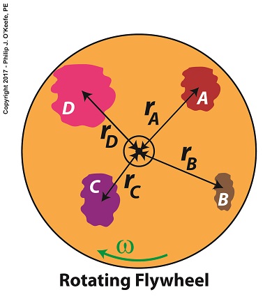
Equation (4) is a great place to begin to calculate the amount of kinetic energy contained within a spinning flywheel, however it is just a beginning, because a flywheel contains many parts. Each of those parts has its own mass, m, and is a unique distance, r, from the flywheel’s center of rotation, and all these parts must be accounted for in order to arrive at a calculation for the total amount of kinetic energy contained within a spinning flywheel.
How Much Kinetic Energy is Contained Within a Spinning Flywheel?
Put another way, we must add together all the m × r2 terms for each and every part of the entire flywheel. How many parts are we speaking of? Well, that depends on the type of flywheel. We’ll discuss that in detail later, after we define a phenomenon that influences the kinetic energy of a flywheel known as the moment of inertia.
For now, let’s just consider the flywheel’s parts in general terms. A general formula to compute the kinetic energy contained within the totality of a spinning flywheel is,
KE = ½ × ∑[m × r2] × ω2 (5)
We’ll discuss the significance of each of these variables next time when we arrive at a method to calculate the kinetic energy contained within all the many parts of a spinning flywheel
.
Copyright 2017 – Philip J. O’Keefe, PE
Engineering Expert Witness Blog
____________________________________ |
Tags: angular velocity, center of rotation, engineering, flywheel, kinetic energy, linear velocity, mass, moment of inertia
Posted in Engineering and Science, Expert Witness, Forensic Engineering, Innovation and Intellectual Property, Personal Injury, Product Liability, Professional Malpractice | Comments Off on How Much Kinetic Energy is Contained Within a Spinning Flywheel?
Thursday, October 19th, 2017
|
Anyone who has spun a potter’s wheel is appreciative of the smooth motion of the flywheel upon which they form their clay, for without it the bowl they’re forming would display irregularities such as unattractive bumps. The flywheel’s smooth action comes as a result of kinetic energy, the energy of motion, stored within it. We’ll take another step towards examining this phenomenon today when we take our first look at calculating this kinetic energy. To do so we’ll make reference to the two types of velocity associated with a spinning flywheel, angular velocity and linear velocity, both of which engineers must negotiate anytime they deal with rotating objects.
Let’s begin by referring back to the formula for calculating kinetic energy, KE. This formula applies to all objects moving in a linear fashion, that is to say, traveling a straight path. Here it is again,
KE = ½ × m × v2
where m is the moving object’s mass and v its linear velocity.
Flywheels rotate about a fixed point rather than move in a straight line, but determining the amount of kinetic energy stored within a spinning flywheel involves an examination of both its angular velocity and linear velocity. In fact, the amount of kinetic energy stored within it depends on how fast it rotates.
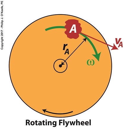
For our example we’ll consider a spinning flywheel, which is basically a solid disc. For our illustrative purposes we’ll divide this disc into hypothetical parts, each having a mass m located a distance r from the flywheel’s center of rotation. We’ll select a single part to examine and call that A.
Two Types of Velocity Associated With a Spinning Flywheel
Part A has a mass, mA, and is located a distance rA from the flywheel’s center of rotation. As the flywheel spins, part A rides along with it at an angular velocity, ω, following a circular path, shown in green. It also moves at a linear velocity, vA, shown in red. vA represents the linear velocity of part A measured at any point tangent to its circular path. This linear velocity would become evident if part A were to become disengaged from the flywheel and cast into the air, whereupon its trajectory would follow a straight line tangent to its circular path.
The linear and angular velocities of part A are related by the formula,
vA = rA × ω
Next time we’ll use this equation to modify the basic kinetic energy formula so that it’s placed into terms that relate to a flywheel’s angular velocity. This will allow us to define a phenomenon at play in the flywheel’s rotation, known as the moment of inertia.
Copyright 2017 – Philip J. O’Keefe, PE
Engineering Expert Witness Blog
____________________________________ |
Tags: angular velocity, energy stored, engineering, flywheel, kinetic energy, linear velocity, mass, moment of inertia, spinning flywheel
Posted in Engineering and Science, Expert Witness, Forensic Engineering, Innovation and Intellectual Property, Personal Injury, Product Liability, Professional Malpractice | Comments Off on Two Types of Velocity Associated With a Spinning Flywheel
Tuesday, October 10th, 2017
|
Last time we introduced angular velocity with regard to flywheels and how a fixed point riding piggyback on a moving flywheel travels the same circular path as its host at a pace that’s measured in units of degrees per second. Today we’ll introduce another unit of measure, the radian, and see how it’s uniquely used to measure angles of circular motion in units of radians per second.
Radians and the Angular Velocity of a Flywheel
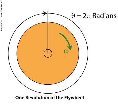
Back in elementary school we worked with protractors and measured angles in degrees, and we were all too familiar with the fact that the average protractor maxed out at 180, or half the degrees present in a complete circle. But in the grownup worlds of physics and engineering, angles of circular motion are measured in units called radians, an international standard equal to 57.3 degrees that’s used to measure objects rotating in circular motion.
If we divide a circle’s value of 360 degrees by the 57.3 degrees that represent a radian, we find there are 6.28 radians in a circle, and oddly enough, it just so happens that 6.28 is equal to 2 × π. Anyone who stayed awake during math class can’t help but remember that π represents a constant value of 3.14, a number that pops up anytime you divide the circumference of a circle by its diameter. No matter the circle’s size, π will always result when you perform this operation.
Applying these facts to radians, we find that during one complete revolution of a flywheel the measure of the angle θ increases from 0 radians to 2π radians.
Suppose we have a flywheel spinning at N revolutions per minute, or RPMs. To calculate the angular velocity, ω, of any point on the flywheel, or the whole wheel for that matter, we use the following formula which provides an answer in radians per second,
ω = [2 × π × N ] ÷ 60 seconds/minute (1)
If a flywheel spins at 3000 RPM, its angular velocity is calculated as,
ω = [2 × π × (3000 RPM)] ÷ 60 seconds/minute (2)
ω = 314.16 radians/second (3)
Next time we’ll see how angular velocity is used to determine the kinetic energy contained within a flywheel.
Copyright 2017 – Philip J. O’Keefe, PE
Engineering Expert Witness Blog
____________________________________ |
Tags: angular velocity, degrees, engineering, flywheel, kinetic energy, radians, revolutions per minute, RPM
Posted in Engineering and Science, Expert Witness, Forensic Engineering, Innovation and Intellectual Property, Personal Injury, Product Liability | Comments Off on Radians and the Angular Velocity of a Flywheel
Wednesday, October 4th, 2017
|
We introduced the flywheel in our last blog and the fact that as long as it’s spinning it acts as a kinetic energy storage device. Today we’ll work our way towards an understanding of how this happens when we discuss angular velocity.
Angular velocity is represented in engineering and physics by the symbol, ω, the Greek letter Omega. The term angular is used to denote physical quantities measured with respect to an angle, especially those quantities associated with rotation.
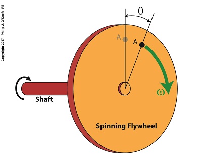
Angular Velocity of a Flywheel
To understand how angular velocity manifests let’s consider a fixed point on the face of a flywheel, represented in the illustration as A. When the flywheel is at rest, point A is in the 12 o’clock position, and as it spins A travels clockwise in a circular path. An angle, θ, is formed as A’s position follows along with the rotation of the flywheel. The angle increases in size as A travels further from its starting point. If A moves one complete revolution, θ will equal 360 degrees, or the total number of degrees present in a circle.
As the flywheel spins through its first revolution into its second, point A travels past its point of origination, and in two complete revolutions it will travel 2 × 360, or 720 degrees, in three revolutions 3 × 360, or 1080 degrees, and so forth. The degrees A travels continue to increase with each revolution of the flywheel.
Angular velocity represents the total number of degrees A travels within a given time period. If we measure the flywheel’s rotational speed with a tachometer and find it takes one second to make 50 revolutions, point A will have traveled the circumference of its path fifty times, and A’s angular velocity would be calculated as,
ω = (50 revolutions per second) × (360 degrees per revolution)
ω = 18,000 degrees per second
Next time we’ll introduce a unit of measurement known as radians which is uniquely used to measuring the angles of circular motion.
Copyright 2017 – Philip J. O’Keefe, PE
Engineering Expert Witness Blog
____________________________________ |
Tags: angular velocity, energy storage, engineering, flywheel, kinetic energy
Posted in Engineering and Science, Expert Witness, Forensic Engineering, Innovation and Intellectual Property, Personal Injury, Product Liability | Comments Off on Angular Velocity of a Flywheel
Monday, September 25th, 2017
|
What came first? The wheel or the flywheel? Archeologists have been debating this question for decades. One thing is certain, they both date back to prehistoric times.
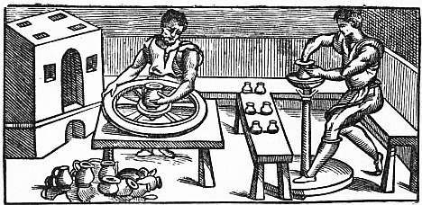
What Came First? The Wheel or the Flywheel?
One of the oldest flywheel discoveries was a potter’s wheel, used to make pottery. It’s a turntable made of stone or heavy wood that’s connected to a massive wheel by a spinning shaft. Once the potter got the flywheel spinning with his hand or foot, the wheel’s heavy weight kept it in virtual perpetual motion, allowing the potter to concentrate on forming the clay he shaped with his hands.
A potter’s wheel, or any other flywheel for that matter, takes a lot of initial effort to put into motion. In other words, the potter must put a lot of his own muscles’ mechanical energy into the flywheel to get it moving. That’s because its sheer weight binds it to the Law of Inertia and makes it want to stay at rest.
But once the flywheel is in motion, the potter’s mechanical energy input is transformed into kinetic energy, the energy of motion. The kinetic energy the potter produces by his efforts results in surplus energy stored within the flywheel. Hence, the flywheel serves as a kinetic energy storage device, similar to a battery which stores electrical energy. As long as the flywheel remains in motion, this stored energy will be used to keep the turntable spinning, which results in no additional mechanical energy needing to be exerted by the potter while forming pots.
The flywheel’s stored energy also makes it hard to stop once it’s in motion. But eventually the frictional force between the potter’s hands and the clay he works drains off all stored kinetic energy.
Since the Industrial Revolution flywheels have been used to store kinetic energy to satisfy energy demands and provide a continuous output of power, which increases mechanical efficiency.
Next time we’ll begin our exploration into the science behind flywheels and see how they’re used in diverse engineering applications.
Copyright 2017 – Philip J. O’Keefe, PE
Engineering Expert Witness Blog
____________________________________ |
Tags: energy storage, engineering, flywheel, frictional force, inertia, kinetic energy, mechanical energy
Posted in Engineering and Science, Expert Witness, Forensic Engineering, Innovation and Intellectual Property, Personal Injury, Product Liability | Comments Off on What Came First? The Wheel or the Flywheel?
Monday, September 4th, 2017
|
We’ve been working our way towards developing values for variables in our example pulley-belt assembly, and last time we calculated the velocity of the belt in that assembly to be 237.99 feet per minute. But before we can go on to calculate the belt’s loose side tension, T2, and tight side tension, T1, we’ll need to discuss unit conversion, specifically how to convert horsepower into foot-pounds per second.
Our working formula for this demonstration is the formula for mechanical power, P, previously introduced and shown again here,
P = (T1 – T2) × V (1)
By engineering convention mechanical power is normally measured in units of foot-pounds per second. But if you’ll recall from a past blog in which we determined the belt’s velocity, V, it was measured in units of feet per minute, not per second.
To further complicate things, the difference in belt tensions, T1 – T2, is stated in units of pounds, and combining these elements together results in P being expressed in foot-pounds per minute, not the required per second, because we are multiplying feet per minute by pounds. That’s a whole lot of unit changing within a single equation, which makes for an awkward situation.
To smooth things out we’ll have to do some converting of units. We’ll start by dividing V by 60 seconds per minute so it can be expressed in units of feet per second,
V = 237.99 feet per minute ÷ 60 seconds per minute (2)
V = 3.93 feet/second (3)
The power in our belt was previously given as 4 horsepower, which must also undergo conversion and be put in terms of foot-pounds per second so it can be used in equation (1).

Unit Conversion, Horsepower to Foot-Pounds per Second
One horsepower is equal to 550 foot-pounds per second, which makes the amount of power, P, in our pulley-belt assembly equal to 2,200 foot-pounds per second.
Units converted, we can now insert the values for V and P into equation (1) to arrive at,
2,200 foot pounds per second = (T1 – T2) × 3.93 feet/second (4)
Next time we’ll use this relationship to develop values for T1 and T2, the belt’s tight and loose side tensions.
Copyright 2017 – Philip J. O’Keefe, PE
Engineering Expert Witness Blog
____________________________________ |
Tags: belt, belt and pulley assembly, belt velocity, engineering, foot pounds per second, horsepower, loose side tension, mechanical power, pulley, tight side tension, unit conversions, units
Posted in Engineering and Science, Expert Witness, Forensic Engineering, Innovation and Intellectual Property, Personal Injury, Product Liability | Comments Off on Unit Conversion, Horsepower to Foot-Pounds per Second
Saturday, July 29th, 2017
|
Last time we determined the value for one of the key variables in the Euler-Eytelwein Formula known as the angle of wrap. To do so we worked with the relationship between the two tensions present in our example pulley-belt assembly, T1 and T2. Today we’ll use physics to solve for T2 and arrive at the Mechanical Power Formula, which enables us to compute the amount of power present in our pulley and belt assembly, a common engineering task.
To start things off let’s reintroduce the equation which defines the relationship between our two tensions, the Euler-Eytelwein Formula, with the value for e, Euler’s Number, and its accompanying coefficients, as determined from our last blog,
T1 = 2.38T2 (1)
Before we can calculate T1 we must calculate T2. But before we can do that we need to discuss the concept of power.
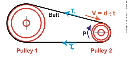
The Mechanical Power Formula in Pulley and Belt Assemblies
Generally speaking, power, P, is equal to work, W, performed per unit of time, t, and can be defined mathematically as,
P = W ÷ t (2)
Now let’s make equation (2) specific to our situation by converting terms into those which apply to a pulley and belt assembly. As we discussed in a past blog, work is equal to force, F, applied over a distance, d. Looking at things that way equation (2) becomes,
P = F × d ÷ t (3)
In equation (3) distance divided by time, or “d ÷ t,” equals velocity, V. Velocity is the distance traveled in a given time period, and this fact is directly applicable to our example, which happens to be measured in units of feet per second. Using these facts equation (3) becomes,
P = F × V (4)
Equation (4) contains variables that will enable us to determine the amount of mechanical power, P, being transmitted in our pulley and belt assembly.
The force, F, is what does the work of transmitting mechanical power from the driving pulley, pulley 2, to the passive driven pulley, pulley1. The belt portion passing through pulley 1 is loose but then tightens as it moves through pulley 2. The force, F, is the difference between the belt’s tight side tension, T1, and loose side tension, T2. Which brings us to our next equation, put in terms of these two tensions,
P = (T1 – T2) × V (5)
Equation (5) is known as the Mechanical Power Formula in pulley and belt assemblies.
The variable V, is the velocity of the belt as it moves across the face of pulley 2, and it’s computed by yet another formula. We’ll pick up with that issue next time.
Copyright 2017 – Philip J. O’Keefe, PE
Engineering Expert Witness Blog
____________________________________ |
Tags: belt, distance divided by time, engineering, Euler-Eytelwein Formula, Euler's Number, force, loose side tension, mechanical power, mechanical power formula, power, power transmitted, pulley, tight side tension, velocity, work
Posted in Engineering and Science, Expert Witness, Forensic Engineering, Innovation and Intellectual Property, Personal Injury, Product Liability | Comments Off on The Mechanical Power Formula in Pulley and Belt Assemblies
Tuesday, June 13th, 2017
|
Last week we saw how friction coefficients as used in the Euler-Eyelewein Formula, can be highly specific to a specialized application, U.S. Navy ship capstans. In fact, many diverse industries benefit from aspects of the Euler-Eytelwein Formula. Today we’ll introduce another engineering application of the Formula, exploring its use within the irrigation system of a hydroponics plant.
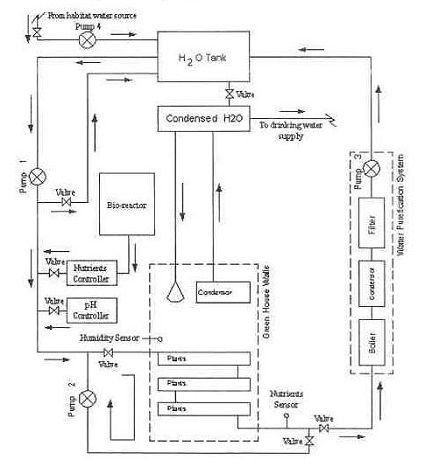
Another Specialized Application of the Euler-Eyelewein Formula
Pumps conveying water are an indispensable part of a hydroponics plant. In the schematic shown here they are portrayed by the symbol ⊗.
In our simplified scenario to be presented next week, these pumps are powered by a mechanical power transmission system, each consisting of two pulleys and a belt. One pulley is connected to a water pump, the other pulley to a gasoline engine. A belts runs between the pulleys to deliver mechanical power from the engine to the pump.
The width of the belts is a key component in an efficiently running hydroponics plant. We’ll see how and why that’s so next time.
Copyright 2017 – Philip J. O’Keefe, PE
Engineering Expert Witness Blog
____________________________________ |
Tags: belt, belt width, coefficient of friction, engineering, Euler-Etytelwein Formula, gasoline engine, hydroponics, mechanical power transmission, power, pulley, pump
Posted in Engineering and Science, Expert Witness, Forensic Engineering, Innovation and Intellectual Property, Personal Injury, Product Liability, Professional Malpractice | Comments Off on Another Specialized Application of the Euler-Eyelewein Formula
Sunday, June 4th, 2017
|
We’ve been talking about pulleys for awhile now, and last week we introduced the term friction coefficient, numerical values derived during testing which quantify the amount of friction present when different materials interact. Friction coefficients for common materials are routinely presented in engineering texts like Marks’ Standard Handbook for Mechanical Engineers. But there are circumstances when more specificity is required, such as when the U.S. Navy, more specifically the Navy Material Command, tested the interaction between various synthetic ropes and ship capstans and developed their own specialized friction coefficients in the process.
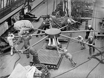
Navy Capstans and the Development of Specialized Friction Coefficients
Capstans are similar to pulleys but have one key difference, they’re made so rope can be wound around them multiple times. When the Navy set out to determine which synthetic rope worked best with their capstans, they did testing and developed highly specialized friction coefficients in the process. This research was at one time Top Secret but has now been declassified. To read more about it, follow this link to the actual handbook:
https://archive.org/stream/DTIC_ADA036718#page/n0/mode/2up
Copyright 2017 – Philip J. O’Keefe, PE
Engineering Expert Witness Blog
____________________________________ |
Tags: capstan, engineering, friction, friction coefficient, pulley, rope
Posted in Engineering and Science, Expert Witness, Forensic Engineering, Innovation and Intellectual Property, Personal Injury, Product Liability | Comments Off on Navy Capstans and the Development of Specialized Friction Coefficients
Sunday, May 14th, 2017
|
Last time we introduced some of the variables in the Euler-Eytelwein Formula, an equation used to examine the amount of friction present in pulley-belt assemblies. Today we’ll explore its two tension-denoting variables, T1 and T2.
Here again is the Euler-Eytelwin Formula,where, T1 and T2 are belt tensions on either side of a pulley,
T1 = T2 × e(μθ)
T1 is known as the tight side tension of the assembly because, as its name implies, the side of the belt containing this tension is tight, and that is so due to its role in transmitting mechanical power between the driving and driven pulleys. T2 is the loose side tension because on its side of the pulley no mechanical power is transmitted, therefore it’s slack–it’s just going along for the ride between the driving and driven pulleys.
Due to these different roles, the tension in T1 is greater than it is in T2.
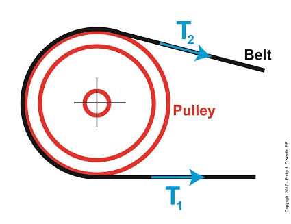
The Two T’s of the Euler-Eytelwein Formula
In the illustration above, tension forces T1 and T2 are shown moving in the same direction, because the force that keeps the belt taught around the pulley moves outward and away from the center of the pulley.
According to the Euler-Eytelwein Formula, T1 is equal to a combination of factors: tension T2 ; the friction that exists between the belt and pulley, denoted as μ; and how much of the belt is in contact with the pulley, namely θ.
We’ll get into those remaining variables next time.
Copyright 2017 – Philip J. O’Keefe, PE
Engineering Expert Witness Blog
____________________________________ |
Tags: belt, belt tension, driven pulley, driving pulley, engineering, Euler-Eytelwein Formula, mechanical power transmission, pulley
Posted in Engineering and Science, Expert Witness, Forensic Engineering, Innovation and Intellectual Property, Personal Injury, Product Liability | Comments Off on The Two T’s of the Euler-Eytelwein Formula